Introduction
This section provides a quickstart to the Taylor-models reachability method with a univariate oscillator as running example. It is a small example that mixes intervals, the sine function, and differential equations. It is easy to check that the function
\[x(t) = x_0 \exp\left(\cos(t) - 1\right),\qquad x_0 ∈ \mathbb{R},\]
solves the following differential equation:
\[x'(t) = -x(t) ~ \sin(t),\qquad t ≥ 0.\]
Standard integration schemes fail to produce helpful solutions if the initial state is an interval. We illustrate this point by solving the given differential equation with the Tsit5 algorithm from OrdinaryDiffEq.jl suite.
using OrdinaryDiffEq, IntervalArithmetic
using IntervalArithmetic.Symbols: (..)

# initial condition
X0 = [-1 .. 1]

# define the problem
function f(dx, x, p, t)
    dx[1] = -x[1] * sin(t)
end

# pass to solvers
prob = ODEProblem(f, X0, (0.0, 2.0))
sol = solve(prob, Tsit5(), adaptive=false, dt=0.05, reltol=1e-6)
Now we plot the result.
using Plots

out = [[interval(sol.t[i]), interval(sol.u[i][1])] for i in 1:20]

fig = plot(out, xlab="t", ylab="x(t)", lw=3.0, alpha=1., c=:black, marker=:none, lab="", title="Standard integrator with an interval initial condition")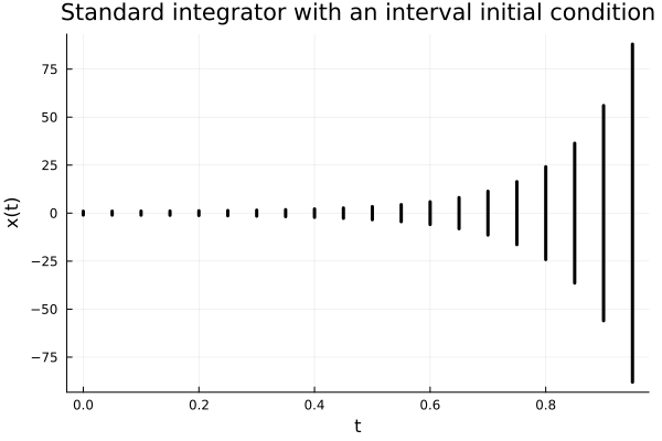
The divergence observed in the solution is due to using an algorithm which doesn't specialize for intervals hence suffers from dependency problems.
However, specialized algorithms can handle this case without noticeable wrapping effect, producing a sequence of sets whose union covers the true solution for all initial points. We use the ReachabilityAnalysis.jl interface to the algorithm TMJets21a, which is itself implemented in TaylorModels.jl.
using ReachabilityAnalysis, Plots

# define the model (same as before)
function f(dx, x, p, t)
    dx[1] = -x[1] * sin(1.0 * t)
end

# define the set of initial states
X0 = Interval(-1.0, 1.0)

# define the initial-value problem
prob = @ivp(x' = f(x), x(0) ∈ X0, dim=1)

# solve it using a Taylor model method
sol = solve(prob, alg=TMJets21a(abstol=1e-10), T=15)

# visualize the solution in time
fig = plot(sol, vars=(0, 1), xlab="t", ylab="x(t)", title="Specialized (Taylor-model based) integrator")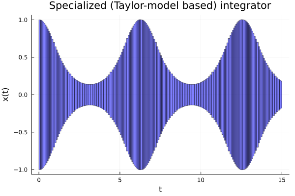
It is illustrative to plot the computed flowpipe and the known analytic solution for a range of initial conditions that cover the range of the initial interval X0 = -1 .. 1. We can do so by overlaying exact solutions taken uniformly from the initial interval.
analytic_sol(x0) = t -> x0 * exp(cos(t) - 1.0)

dt = range(0, 15, length=100)
x0vals = range(-1, 1, length=25)

fig = plot()
plot!(fig, sol, lw=0.0, vars=(0, 1), xlab="t", ylab="x(t)", title="Specialized (Taylor-model based) integrator")
[plot!(fig, dt, analytic_sol(x0).(dt), lab="", c=:magenta, lw=2.0, xlab="t", ylab="x(t)") for x0 in x0vals]
fig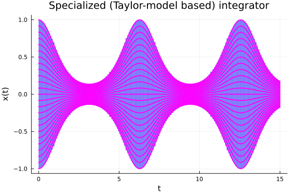
ReachabilityAnalysis.jl defines several methods to analyze the solution. For example, the number of reach-sets can be obtained using length (more generally, use numrsets for hybrid systems):
# number of computed reach-sets
length(sol)172Solutions implement the array interface hence it is possible to index them:
# first reach-set of the flowpipe
sol[1]
TaylorModelReachSet{Float64, Float64}(TaylorModels.TaylorModel1{TaylorN{Float64}, Float64}[ 1.0 x₁ + ( - 0.5 x₁) t² + ( 0.16666666666666666 x₁) t⁴ + ( - 0.04305555555555555 x₁) t⁶ + ( 0.009399801587301585 x₁) t⁸ + [-1.15691e-20, 1.15691e-20]], ReachabilityAnalysis.TimeInterval{IntervalArithmetic.Interval{Float64}}([0.0, 0.100777]))Note that sol[1] is an expansion in time whose coefficients are polynomials in space. The associated time span can be obtained with tspan:
# time span of this reach-set
tspan(sol[1])
ReachabilityAnalysis.TimeInterval{IntervalArithmetic.Interval{Float64}}([0.0, 0.100777])Similarly we can print the last reach-set:
sol[end]TaylorModelReachSet{Float64, Float64}(TaylorModels.TaylorModel1{TaylorN{Float64}, Float64}[ 0.1779576289788848 x₁ + ( - 0.12234109170162545 x₁) t + ( 0.10667039458327013 x₁) t² + ( - 0.033669261864646166 x₁) t³ + ( 0.009254898907687442 x₁) t⁴ + ( 0.0031126156317747805 x₁) t⁵ + ( - 0.002553610888200177 x₁) t⁶ + ( 0.0010923362551788728 x₁) t⁷ + ( - 0.00014851535275118348 x₁) t⁸ + [-4.16068e-10, 4.16068e-10]], ReachabilityAnalysis.TimeInterval{IntervalArithmetic.Interval{Float64}}([14.9499, 15.0]))tspan(sol[end])ReachabilityAnalysis.TimeInterval{IntervalArithmetic.Interval{Float64}}([14.9499, 15.0])It is also possible to filter solutions by the time variable using parentheses:
# find the reach-set(s) that contain 1.0 in their time span
aux = sol(1.0)
TaylorModelReachSet{Float64, Float64}(TaylorModels.TaylorModel1{TaylorN{Float64}, Float64}[ 0.6411129385689787 x₁ + ( - 0.533117272147243 x₁) t + ( 0.04360354980682554 x₁) t² + ( 0.17547343154298664 x₁) t³ + ( - 0.08311004314689788 x₁) t⁴ + ( - 0.016358794254811418 x₁) t⁵ + ( 0.025377422836099808 x₁) t⁶ + ( - 0.004089907943834324 x₁) t⁷ + ( - 0.0040021378768007486 x₁) t⁸ + [-2.38073e-11, 2.38073e-11]], ReachabilityAnalysis.TimeInterval{IntervalArithmetic.Interval{Float64}}([0.981891, 1.06367]))tspan(aux)ReachabilityAnalysis.TimeInterval{IntervalArithmetic.Interval{Float64}}([0.981891, 1.06367])Filtering by the time span also works with time intervals; in the following example, we obtain all reach-sets whose time span with the interval 1.0 .. 3.0 is non-empty:
length(sol(1.0 .. 3.0))22On the other hand, evaluating over a given time point or time interval can be achieved using the evaluate function:
# evaluate over the full time interval ≈ [0, 0.100777]
evaluate(sol[1], tspan(sol[1]))
1-element Vector{TaylorModels.TaylorModelN{1, Float64, Float64}}:
0.9974610138195609 x₁ + [-0.00253899, 0.00253899]# evaluate over the final time point 0.10077670723811318
evaluate(sol[1], tend(sol[1]))1-element Vector{TaylorModels.TaylorModelN{1, Float64, Float64}}:
0.9949391731732371 x₁ + [-1.11034e-16, 1.11034e-16]# evaluate the final reach-set at the final time point
evaluate(sol[end], 15.0)1-element Vector{TaylorModels.TaylorModelN{1, Float64, Float64}}:
0.17209856519153915 x₁ + [-4.16068e-10, 4.16068e-10]Finally, note that the solution structure, apart from storing the resulting flowpipe, contains information about the algorithm that was used to obtain it:
sol.algTMJets21a{Float64, ZonotopeEnclosure}
orderQ: Int64 2
orderT: Int64 8
abstol: Float64 1.0e-10
maxsteps: Int64 2000
adaptive: Bool true
minabstol: Float64 1.0e-50
absorb: Bool false
disjointness: ZonotopeEnclosure ZonotopeEnclosure()
The type of reach-set representation as well as the set representation can be obtained using rsetrep and setrep respectively.
# type of the reach-set representation
rsetrep(sol)TaylorModelReachSet{Float64}# type of the set representation
setrep(sol)Vector{TaylorModel1{TaylorN{Float64}, Float64}} (alias for Array{TaylorModels.TaylorModel1{TaylorN{Float64}, Float64}, 1})The following section discusses more details about those representations.