Set propagation in dense time

In this section we transition from the discrete time problem considered before to a problem in which time is assumed to be a continuously varying quantity. Thus, our next "toy" problem is the system of ordinary differential equations that describe a simple, undamped, harmonic oscillator:

\[\begin{aligned} x'(t) &= y(t) \\ y'(t) &= -x(t) \end{aligned} \qquad \textrm{subject to } (x(0), y(0)) ∈ X_0 = [0.8, 1.2] \times [0.8, 1.2] ⊆ \mathbb{R}^2\]

We are interested in solving this problem for all $t ∈ [0, T]$ with $T = 2π$.

The problem studied in the previous section is the "discrete analogue" of the purely continuous system of differential equations defined above.

The matrix $M(ω t)$ describes the solution of a mathematical model called simple harmonic oscillator with natural frequency $ω = 1$, and the analytic solution is

\[\begin{aligned} x(t) &= x_0 \cos~ t + y_0 \sin~ t \\ y(t) &= -x_0 \sin t + y_0 \cos t \end{aligned}\]

Observe that $(x(t), y(t))^T$ is just the matrix $M(t)$ applied to the initial state $(x_0, y_0)^T$.

Define the invariant $G: \{(x, y) ∈ \mathbb{R}^2: x ≥ 1.3 \}$.

using ReachabilityAnalysis, Plots
using ReachabilityAnalysis: center



# initial states
X0 = BallInf(ones(2), 0.2)

# rotation matrix
M(θ) = [cos(θ) sin(θ); -sin(θ) cos(θ)]

# analytic solution to visualize the solution at intermediate times

samples = sample(X0, 200, include_vertices=true)
tt = range(0, 2pi/20, length=100)

F = [ReachSet(linear_map(M(ti), X0), ti) for ti in range(0, 2pi, step=2pi/20)]

fig = plot(F[1], vars=(1, 2), lab="X0", c=:blue)
plot!(fig, F[2], vars=(1, 2), lab="Φ * X0", c=:orange)
[plot!(fig, xcoords, ycoords, seriestype=:path, lab="", c=:magenta, ratio=1.) for (xcoords, ycoords) in analytic_sol.(samples, Ref(tt))]
fig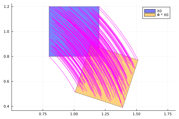

Conservative time discretization

fig = plot()

plot!(fig, convexify(F[1:2]), vars=(1, 2), ls=:dash, lw=3.0, c=:green, lab="CH(X0, Φ*X0)")
plot!(fig, F[1], vars=(1, 2), lab="X0", c=:blue)
plot!(fig, F[2], vars=(1, 2), lab="Φ*X0", c=:orange)
[plot!(fig, xcoords, ycoords, seriestype=:path, lab="", c=:magenta, ratio=1.) for (xcoords, ycoords) in analytic_sol.(samples, Ref(tt))]

fig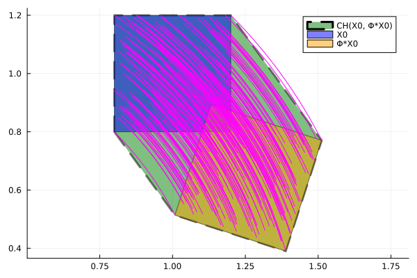

xlims!(1.0, 1.5)
ylims!(0.8, 1.2)

Algorithms implementing conservative time discretization can be used from the discretize(ivp::IVP, δ, alg::ReachabilityAnalysis.DiscretizationModule.AbstractApproximationModel) function. Set-based conservative discretization of a continuous-time initial value problem into a discrete-time problem. This function receives three inputs: the initial value problem (ivp) for a linear ODE in canonical form, (e.g. the system returned by normalize); the step-size (δ), and the algorithm (alg) used to compute the approximation model. Do subtypes(ReachabilityAnalysis.DiscretizationModule.AbstractApproximationModel) to see the available approximation models.

The output of a discretization is a new initial value problem of a discrete system. Different approximation algorithms and their respective options are described in the docstring of each method, e.g. Forward.

Initial-value problems considered in this function are of the form

\[x' = Ax(t) + u(t),\qquad x(0) ∈ \mathcal{X}_0,\qquad (1)\]

and where $u(t) ∈ U(k)$ add where $\{U(k)\}_k$ is a sequence of sets of non-deterministic inputs and $\mathcal{X}_0$ is the set of initial states. Recall that this initial-value problem is called homogeneous whenever U is the empty set. Other problems, e.g. $x' = Ax(t) + Bu(t)$ can be brought to the canonical form with the function normalize.

The initial value problem returned by this function consists of a set discretized (also called bloated) initial states $Ω₀$, together with the coefficient matrix $Φ = e^{Aδ}$ and a transformed sequence of inputs if $U$ is non-empty.

Two main variations of this algorithm are considered: dense time case and discrete time case.

• In the dense time case, the transformation is such that the trajectories

of the given continuous system are included in the computed flowpipe of the discretized system. More precisely, given a step size $δ$ and the system (1) conservative set-based discretization function computes a set, $Ω₀$, that guarantees to contain all the trajectories of (1) starting at any $x(0) ∈ \mathcal{X}_0$ and for any input function that satisfies $u(t) ∈ U(1)$, for any $t ∈ [0, δ]$. If $U$ is time-varying, this function also discretizes the inputs for $k ≥ 0$.

• In the discrete time case, there is no bloating of the initial states and the

input is assumed to remain constant between sampled times. Use the algorithm NoBloating() for this setting. If $U$ is time-varying, this function also discretizes the inputs for $k ≥ 0$.

There are algorithms to obatin such transformations, called approximation models in the technical literature. For references to the original papers, see the docstring of each concrete subtype of AbstractApproximationModel.