SEIR

Model description

The SEIR model is an compartmental model. These try to predict things such as how a disease spreads, or the total number infected, or the duration of an epidemic, and to estimate various epidemiological parameters such as the reproductive number. The dynamics are described as follows:

\[\begin{aligned} \dot{S} &= β I S \\ \dot{E} &= β I S - α E \\ \dot{I} &= -γ I - α E \\ \dot{R} &= γ I \end{aligned}\]

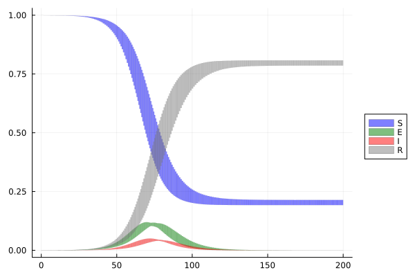
where $S$ is the stock of susceptible population, $E$ is the stock of exposed population, $I$ is the stock of infected, $R$ is the stock of removed population (either by death or recovery), with $S + E + I + R = N$.

using ReachabilityAnalysis

@taylorize function seir!(dx, x, p, t)
    S, E, I, R, α, β, γ = x

    βIS = β * (I * S)
    αE = α * E
    γI = γ * I

    dx[1] = -βIS      # dS
    dx[2] = βIS - αE  # dE
    dx[3] = -γI + αE  # dI
    dx[4] = γI        # dR

    # uncertain parameters
    dx[5] = zero(α)
    dx[6] = zero(β)
    dx[7] = zero(γ)
    return dx
end

Specification

The initial condition is $E₀ = 1e-4$, $x₀ = [1-E₀, E₀, 0, 0]$, $α = 0.2 ± 0.01$, $β = 1.0 ± 0.0$, $γ = 0.5 ± 0.01$, and $p = [α, β, γ]$. The time horizon is $200$.

E₀ = 1e-4
x₀ = [1 - E₀, E₀, 0, 0]
α = 0.2 ± 0.01
β = 1.0 ± 0.0
γ = 0.5 ± 0.01
p = [α, β, γ]
X0 = IntervalBox(vcat(x₀, p));
prob = @ivp(x' = seir!(x), dim:7, x(0) ∈ X0);

Analysis

sol = solve(prob; T=200.0, alg=TMJets21a(; orderT=7, orderQ=1))
solz = overapproximate(sol, Zonotope);

Results

using Plots

fig = plot(; legend=:outerright)
plot!(fig, solz; vars=(0, 1), color=:blue, lw=0.0, lab="S")
plot!(fig, solz; vars=(0, 2), color=:green, lw=0.0, lab="E")
plot!(fig, solz; vars=(0, 3), color=:red, lw=0.0, lab="I")
plot!(fig, solz; vars=(0, 4), color=:grey, lw=0.0, lab="R")