Building

Model description

The model corresponds to a building (the Los Angeles University Hospital) with 8 floors, each having 3 degrees of freedom, namely displacements in $x$ and $y$ directions, and rotation ^[ASG00]. These 24 variables evolve according to

\[ M\ddot{q}(t) + C\dot{q}(t) + Kq(t) = vu(t),\]

where $u(t)$ is the input. This system can be put into a traditional state-space form of order 48 by defining $x = (q, \dot{q})^T$. We are interested in the motion of the first coordinate $q_1(t)$, hence we choose $v = (1, 0, \ldots, 0)^T$ and the output $y(t) = \dot{q}_1(t) = x_{25}(t)$. In canonical form,

\[\begin{aligned} \dot{x}(t) &= Ax(t) + Bu(t), \qquad u(t) ∈ \mathcal{U} \\ y(t) &= C x(t) \end{aligned}\]

where $x(t) ∈ \mathbb{R}^{48}$ is the state vector, $\mathcal{U} ⊆ \mathbb{R}$ is the input set, and $A ∈ \mathbb{R}^{48 × 48}$ and $B ∈ \mathbb{R}^{48 × 1}$ are matrices given in the file building.jld2. Here $y(t)$ is the output with $C ∈ \mathbb{R}^{1 × 48}$ being the projection onto the coordinate 25.

There are two versions of this benchmark:

• Time-varying inputs: The inputs can change arbitrarily over time: $\forall t: u(t) ∈ \mathcal{U}$.

• Constant inputs: The inputs are only uncertain in the initial value, and constant over time: $u(0) ∈ \mathcal{U}$, $\dot{u}(t)= 0.$

In both cases, the input set $\mathcal{U}$ is the interval $[0.8, 1.0]$, and the initial states are taken from Table 2.2 in ^[TLT16].

using ReachabilityAnalysis, JLD2, ReachabilityBase.CurrentPath
using ReachabilityBase.Arrays: SingleEntryVector
using ReachabilityAnalysis: add_dimension

const x25 = SingleEntryVector(25, 48, 1.0)
const x25e = SingleEntryVector(25, 49, 1.0)

path = @current_path("Building", "building.jld2")

function building_common()
    @load path A B

    c = [fill(0.000225, 10); fill(0.0, 38)]
    r = [fill(0.000025, 10); fill(0.0, 14); 0.0001; fill(0.0, 23)]
    X0 = Hyperrectangle(c, r)

    U = Interval(0.8, 1.0)

    return A, B, X0, U
end

function building_BLDF01()
    A, B, X0, U = building_common()
    n = size(A, 1)
    S = @system(x' = A * x + B * u, u ∈ U, x ∈ Universe(n))
    prob_BLDF01 = InitialValueProblem(S, X0)
    return prob_BLDF01
end

function building_BLDC01()
    A, B, X0, U = building_common()
    n = size(A, 1)
    Ae = add_dimension(A)
    Ae[1:n, end] = B
    prob_BLDC01 = @ivp(x' = Ae * x, x(0) ∈ X0 × U)
    return prob_BLDC01
end;

Specification

The verification goal is to show that the displacement $y_1$ of the top floor of the building remains below a given bound. In addition to the safety specification from the original benchmark, there are two UNSAT instances that serve as sanity checks to ensure that the model and the tool work as intended. But there is a caveat: In principle, verifying an UNSAT instance only makes sense formally if a witness is provided (counterexample, underapproximation, etc.). We instead run the tool with the same accuracy settings on an SAT-UNSAT pair of instances. The SAT instance demonstrates that the overapproximation is not too coarse, and the UNSAT instance indicates that the overapproximation is indeed conservative.

• BDS01: Bounded time, safe property: For all $t ∈ [0, 20]$, $y_1(t) ≤ 5.1 ⋅ 10^{-3}$. This property is assumed to be satisfied.

• BDU01: Bounded time, unsafe property: For all $t ∈ [0, 20]$, $y_1(t) ≤ 4 ⋅ 10^{-3}$. This property is assumed to be violated. Property BDU01 serves as a sanity check. A tool should be run with the same accuracy settings on BLDF01-BDS01 and BLDF01-BDU01, returning UNSAT on the former and SAT on the latter.

• BDU02: Bounded time, unsafe property: The forbidden states are $\{y_1(t) ≤ -0.78 ⋅ 10^{-3} \wedge t = 20\}$. This property is assumed to be violated for BLDF01 and satisfied for BLDC01. Property BDU02 serves as a sanity check to confirm that time-varying inputs are taken into account. A tool should be run with the same accuracy settings on BLDF01-BDU02 and BLDC01-BDU02, returning UNSAT on the former and SAT on the latter.

Analysis & results

For the discrete-time analysis we use a step size of $0.01$.

using Plots

BLDF01

prob_BLDF01 = building_BLDF01();

Dense time

sol_BLDF01_dense = solve(prob_BLDF01; T=20.0,
                         alg=LGG09(; δ=0.004, vars=(25), n=48))

fig = plot(sol_BLDF01_dense; vars=(0, 25), linecolor=:blue, color=:blue,
           alpha=0.8, lw=1.0, xlab="t", ylab="x25")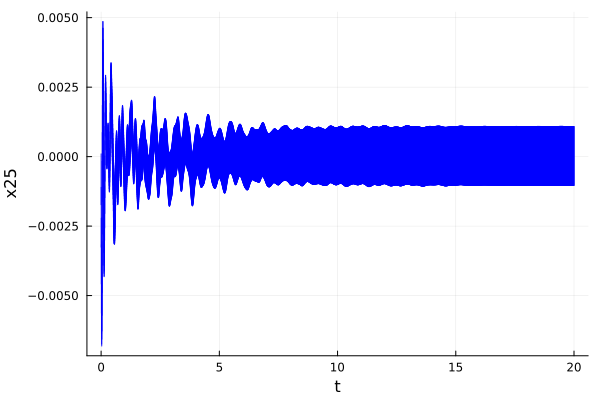

Safety properties:

@assert ρ(x25, sol_BLDF01_dense) <= 5.1e-3 "the property should be proven"  # BLDF01 - BDS01
@assert !(ρ(x25, sol_BLDF01_dense) <= 4e-3) "the property should not be proven"  # BLDF01 - BDU01
ρ(x25, sol_BLDF01_dense)

0.004860238896785233

@assert !(ρ(x25, sol_BLDF01_dense(20.0)) <= -0.78e-3) "the property should not be proven"  # BLDF01 - BDU02
ρ(x25, sol_BLDF01_dense(20.0))

0.0010835336749422345

Discrete time

sol_BLDF01_discrete = solve(prob_BLDF01; T=20.0,
                            alg=LGG09(; δ=0.01, vars=(25), n=48, approx_model=NoBloating()));

fig = plot(sol_BLDF01_discrete; vars=(0, 25), linecolor=:blue, color=:blue,
           alpha=0.8, lw=1.0, xlab="t", ylab="x25")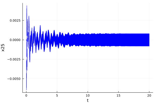

Safety properties:

@assert ρ(x25, sol_BLDF01_discrete) <= 5.1e-3 "the property should be proven"  # BLDF01 - BDS01
@assert !(ρ(x25, sol_BLDF01_discrete) <= 4e-3) "the property should not be proven"  # BLDF01 - BDU01
ρ(x25, sol_BLDF01_discrete)

0.004412266117562393

@assert !(ρ(x25, sol_BLDF01_discrete(20.0)) <= -0.78e-3) "the property should not be proven"  # BLDF01 - BDU02
ρ(x25, sol_BLDF01_discrete(20.0))

0.0007977837510527828

BLDC01

prob_BLDC01 = building_BLDC01();

Dense time

sol_BLDC01_dense = solve(prob_BLDC01; T=20.0, alg=LGG09(; δ=0.005, vars=(25), n=49))

fig = plot(sol_BLDC01_dense; vars=(0, 25), linecolor=:blue, color=:blue,
           alpha=0.8, lw=1.0, xlab="t", ylab="x25")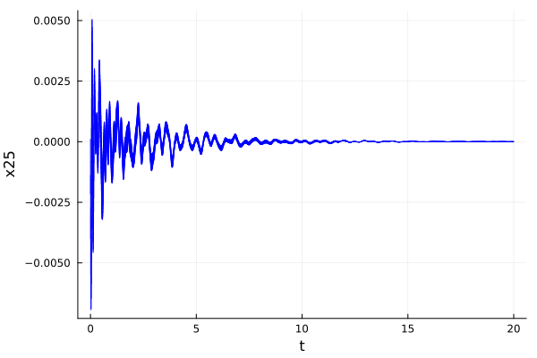

Safety properties

@assert ρ(x25e, sol_BLDC01_dense) <= 5.1e-3 "the property should be proven"  # BLDC01 - BDS01
@assert !(ρ(x25e, sol_BLDC01_dense) <= 4e-3) "the property should not be proven"  # BLDC01 - BDU01
ρ(x25e, sol_BLDC01_dense)

0.00505263426354628

@assert !(ρ(x25e, sol_BLDC01_dense(20.0)) <= -0.78e-3) "the property should not be proven"  # BLDC01 - BDU02
ρ(x25, sol_BLDF01_discrete(20.0))

0.0007977837510527828

Discrete time

sol_BLDC01_discrete = solve(prob_BLDC01; T=20.0,
                            alg=LGG09(; δ=0.01, vars=(25), n=49, approx_model=NoBloating()))

fig = plot(sol_BLDC01_discrete; vars=(0, 25), linecolor=:blue, color=:blue,
           alpha=0.8, lw=1.0, xlab="t", ylab="x25")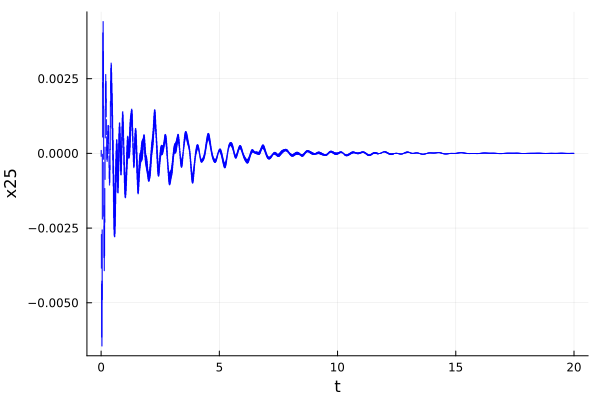

Safety properties

@assert ρ(x25e, sol_BLDC01_discrete) <= 5.1e-3 "the property should be proven" # BLDC01 - BDS01
@assert !(ρ(x25e, sol_BLDC01_discrete) <= 4e-3) "the property should not be proven" # BLDC01 - BDU01
ρ(x25e, sol_BLDC01_discrete)

0.004412266117562392

@assert !(ρ(x25e, sol_BLDC01_discrete(20.0)) <= -0.78e-3) "the property should not be proven" # BLDC01 - BDU02
ρ(x25e, sol_BLDC01_discrete(20.0))

5.582597411711546e-7

References