Square Wave Oscillator

Model description

using ReachabilityAnalysis, Symbolics

function multistable_oscillator(; X0=Interval(0.0, 0.05),
                                V₊=+13.5, V₋=-13.5,
                                R=20.E3, C=5.5556E-8,
                                R1=20.E3, R2=20.E3)
    @variables x
    τ = 1 / (R * C)
    α = R2 / (R1 + R2)
    A = -τ
    automaton = GraphAutomaton(2)

    b = (τ / α) * V₊
    I₊ = HalfSpace(x <= α * V₊)
    m1 = @system(x' = A * x + b, x ∈ I₊)

    b = (τ / α) * V₋
    I₋ = HalfSpace(x >= α * V₋)
    m2 = @system(x' = A * x + b, x ∈ I₋)

    add_transition!(automaton, 1, 2, 1)
    g1 = Hyperplane(x == α * V₊)
    r1 = ConstrainedIdentityMap(1, g1)

    add_transition!(automaton, 2, 1, 2)
    g2 = Hyperplane(x == α * V₋)
    r2 = ConstrainedIdentityMap(1, g2)

    modes = [m1, m2]
    resetmaps = [r1, r2]
    H = HybridSystem(automaton, modes, resetmaps)

    # initial condition in mode 1
    X0e = [(1, X0)]
    return IVP(H, X0e)
end;

Specification

prob = multistable_oscillator();

Analysis

sol = solve(prob; T=100e-4, alg=INT(; δ=1.E-6), fixpoint_check=false);

Below we print the automaton location of each flowpipe segment:

location.(sol)'

1×19 adjoint(::Vector{Int64}) with eltype Int64:
 1  2  1  2  1  2  1  2  1  2  1  2  1  2  1  2  1  2  1

Results

using Plots

old_ztol = LazySets._ztol(Float64)
LazySets.set_ztol(Float64, 1e-8);  # use higher precision for the plots

fig = plot(sol; vars=(0, 1), xlab="t", ylab="v-")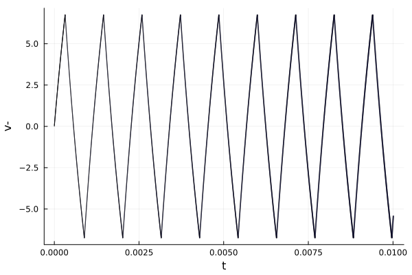

Analyzing the first transition

Let us analyze the first transition in detail. If we plot the last ten reach sets of the first flowpipe, we observe that only the last three actually intersect with the guard:

fig = plot(sol[1][(end - 10):end]; vars=(0, 1), xlab="t", ylab="v-")
plot!(fig, x -> 6.75; xlims=(3.1e-4, 3.3e-4), lab="Guard", lw=2.0, color=:red)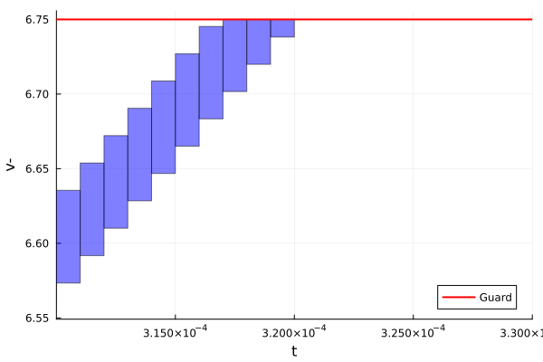

We now cluster those reach sets into a single hyperrectangle:

Xc = cluster(sol[1], [318, 319, 320], BoxClustering(1));

Plotting this set matches with the flowpipe after the jump:

fig = plot(sol[1][(end - 10):end]; vars=(0, 1))
plot!(fig, sol[2][1:10]; vars=(0, 1))
plot!(fig, x -> 6.75; xlims=(3.1e-4, 3.3e-4), lab="Guard", lw=2.0, color=:red)
plot!(fig, Xc[1]; vars=(0, 1), c=:grey)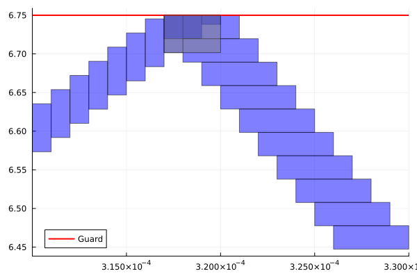

Fixpoint check

Finally, we note that the algorithm can find an invariant of the system after the first period. To activate this check, pass the fixpoint_check=true flag to the solve function. The computation terminates as soon as the last reach set is contained in a previously explored starting set.

sol = solve(prob; T=100e-4, alg=INT(; δ=1.E-6), fixpoint_check=true)
tspan(sol)

[0, 0.00145601]

fig = plot(sol; vars=(0, 1), xlab="t", ylab="v-")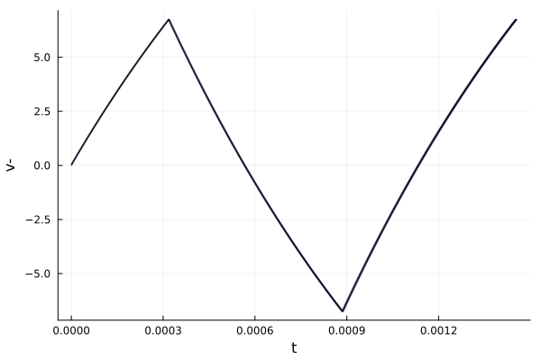

LazySets.set_ztol(Float64, old_ztol);  # reset precision