Van der Pol oscillator

The Van der Pol oscillator was introduced by the Dutch physicist Balthasar van der Pol. This is a famous model, typically investigated in the study of nonlinear dynamics. The model presents non-conservative oscillations with non-linear damping. In the past, it has been of relevance in several practical problems of engineering such as circuits containing vacuum tubes. For more information on the model, see Wikipedia.

Here we compute the evolution of the limit cycle in the phase plane for a set of initial conditions. For this set, we consider a safety property, originally from ^[ARCHCOMP], that there is no solution starting from the initial set that exceeds a prescribed upper bound on the velocity $y(t) := x'(t)$ at all times in the given time span. Moreover, we also illustrate the computation of an invariant set using the obtained flowipe. Finally, we study the limit cycle à la Poincaré by defining a function that computes the cross section of the flowpipe at each revolution. Interestingly, this method gives an algorithmic proof that the safety condition obtained previously is actually verified at all times, i.e. over the unbounded time horizon $[0, ∞)$.

Model description

The dynamics of the Van der Pol oscillator are described by the following differential equations with two variables:

\[\begin{aligned} \dot{x} &= y \\ \dot{y} &= μ (1 - x^2) y - x \end{aligned}\]

The system has a stable limit cycle. This limit cycle becomes increasingly sharp for higher values $μ$. Here we consider the parameter $μ = 1$.

using ReachabilityAnalysis

@taylorize function vanderpol!(du, u, p, t)
    x, y = u
    local μ = 1.0
    du[1] = y
    du[2] = (μ * y) * (1 - x^2) - x
    return du
end

Specification

We set the initial condition $x(0) ∈ [1.25, 1.55]$, $y(0) ∈ [2.35,2.45]$. The unsafe set is given by $y ≥ 2.75$ for a time span $[0, 7]$. In other words, we would like to prove that there does not exist a solution of the model with a $y$ value which is greater than 2.75, for any initial condition from the given domain. The time horizon $T = 7$ is chosen such that the oscillator can do at least one full cycle.

X0 = Hyperrectangle(; low=[1.25, 2.35], high=[1.55, 2.45])
prob = @ivp(x' = vanderpol!(x), dim:2, x(0) ∈ X0);

Analysis

sol = solve(prob; T=7.0, alg=TMJets(; abstol=1e-12));

For further computations, it is convenient to work with a zonotopic overapproximation of the flowpipe.

solz = overapproximate(sol, Zonotope);

The maximum value of variable $y$ is obtained by computing the support function of the flowpipe along direction $[0, 1]$:

y_bound = ρ([0.0, 1.0], solz)
@assert y_bound < 2.75 "the property should be proven"
y_bound

2.724977587223378

This shows that the property is satisfied. Below we plot the flowpipe in the x-y plane, together with the horizontal line $y = 2.75$.

Results

using Plots

fig = plot(solz; vars=(1, 2), lw=0.2, xlims=(-2.5, 2.5), xlab="x", ylab="y")
plot!(x -> 2.75; color=:red, lab="y = 2.75", ls=:dash, legend=:bottomright)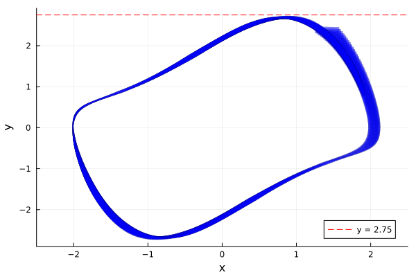

We can also plot the state variables $x(t)$ and $y(t)$ as a function of time (recall that 0 in vars is used to denote the time variable):

fig = plot(solz; vars=(0, 1), lw=0.2, xlab="t", ylab="x")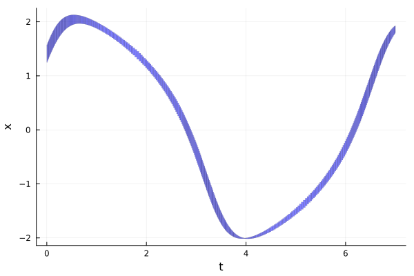

fig = plot(solz; vars=(0, 2), lw=0.2, xlab="t", ylab="y")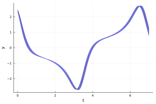

Invariant Set

We can use the reachability result to examine an invariant of the system. In other words, we can algorithmically prove that the flowpipe re-enters from where it started after one loop iteration, using inclusion checks.

fig = plot(solz; vars=(1, 2), lw=0.2, xlims=(0.0, 2.5), ylims=(1.6, 2.8), xlab="x", ylab="y")
plot!(solz[1:13]; vars=(1, 2), color=:green, lw=1, alpha=0.5, lab="F[1:13]")
plot!(solz[388]; vars=(1, 2), color=:red, lw=1, alpha=0.6, lab="F[388]")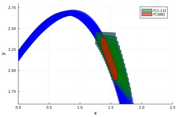

It can be seen that the reach set at index 388 corresponding to the time-span

tspan(solz[388])

[6.74967, 6.7599]

is included in the set union $F[1] ∪ \cdots ∪ F[13]$ of previously computed reach sets. Notice that all future trajectories starting from the 388-th reach set are already covered by the flowpipe. Therefore, we have found an invariant set.

Limit cycle

To examine the limit cycle, we can intersect a line segment perpendicular to the flowpipe, which will allow us to get a cross section of the sets in order to prove that after one cycle the intersection segment actually shrinks. This approach is similar to the method of Poincaré sections.

line = LineSegment([1, 2.0], [2.0, 2.5])
fig = plot(solz; vars=(1, 2), lw=0.2, xlims=(0.0, 2.5), ylims=(1.6, 2.8), xlab="x", ylab="y")
plot!(solz[1:13]; vars=(1, 2), color=:green, lw=1.0, alpha=0.5, lab="F[1:13]")
plot!(solz[388]; vars=(1, 2), color=:red, lw=1.0, alpha=0.6, lab="F[388]")
plot!(line; lw=2.0)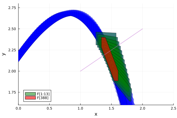

Next, we define a function to get the cross section of the flowpipe. The function needs the flowpipe, a line segment that cuts the flowpipe, and the indices of the subsets to cut.

function cross_section(line::LineSegment, F, idx)
    p = VPolygon()
    for i in idx
        x = intersection(line, set(F[i]))
        if !isempty(x)
            p = convex_hull(p, x)
        end
    end
    vl = vertices_list(p)
    @assert length(vl) == 2
    return LineSegment(vl[1], vl[2])
end;

Then we can get the cross section of the first 13 sets and the last set.

ifirst = cross_section(line, solz, 1:13)
ilast = cross_section(line, solz, [388]);

We can also calculate the length of each cross section.

lfirst = norm(ifirst.q - ifirst.p)

0.28930757953811087

llast = norm(ilast.q - ilast.p)

0.11046336365917839

fig = plot(ifirst; lw=3.0, alpha=1.0, label="First subsets", legend=:bottomright)
plot!(ilast; lw=5.0, alpha=1.0, label="Last subset")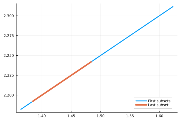

The inclusion check succeeds:

@assert ilast ⊆ ifirst "the cross section should get smaller"

As we can see, the cross section of the last reach set is a subset of the first 13 reach sets. Thus, the cycle will continue, presumably getting smaller each revolution.

References