Quadrotor

Model description

We study the dynamics of a quadrotor, derived in ^[B08] and used in ^[GSA21]. Starting with the state variables, we have the inertial (north) position $x_1$, the inertial (east) position $x_2$, the altitude $x_3$, the longitudinal velocity $x_4$, the lateral velocity $x_5$, the vertical velocity $x_6$, the roll angle $x_7$, the pitch angle $x_8$, the yaw angle $x_9$, the roll rate $x_{10}$, the pitch rate $x_{11}$, and the yaw rate $x_{12}$. We further require the following parameters: gravity constant $g = 9.81$ [m/s$^2$], radius of center mass $R = 0.1$ [m], distance of rotors to center mass $l = 0.5$ [m], rotor mass $M_{rotor} = 0.1$ [kg], center mass $M = 1$ [kg], and total mass $m = M + 4M_{rotor}$.

From the above parameters, we can compute the moments of inertia as

\[\begin{aligned} J_x &= 0.4 M R^2 + 2 l^2 M_{rotor}, \\ J_y &= J_x, \\ J_z &= 0.4 M R^2 + 4 l^2 M_{rotor}. \end{aligned}\]

Finally, we can write the set of ordinary differential equations for the quadrotor according to ^[B08] (Eq. (16)-(19)):

\[\begin{aligned} \dot{x}_1 &= \cos(x_8)\cos(x_9)x_4 + \Big(\sin(x_7)\sin(x_8)\cos(x_9) - \cos(x_7)\sin(x_9)\Big)x_5 \\ &~~~ + \Big(\cos(x_7)\sin(x_8)\cos(x_9) + \sin(x_7)\sin(x_9)\Big)x_6 \\ \dot{x}_2 &= \cos(x_8)\sin(x_9)x_4 + \Big(\sin(x_7)\sin(x_8)\sin(x_9) + \cos(x_7)\cos(x_9)\Big)x_5 \\ &~~~ + \Big(\cos(x_7)\sin(x_8)\sin(x_9) - \sin(x_7)\cos(x_9)\Big)x_6 \\ \dot{x}_3 &= \sin(x_8)x_4 - \sin(x_7)\cos(x_8)x_5 - \cos(x_7)\cos(x_8)x_6 \\ \dot{x}_4 &= x_{12}x_5 - x_{11}x_6 - g\sin(x_8) \\ \dot{x}_5 &= x_{10}x_6 - x_{12}x_4 + g\cos(x_8)\sin(x_7) \\ \dot{x}_6 &= x_{11}x_4 - x_{10}x_5 + g\cos(x_8)\cos(x_7) - \dfrac{F}{m} \\ \dot{x}_7 &= x_{10} + \sin(x_7)\tan(x_8)x_{11} + \cos(x_7)\tan(x_8)x_{12} \\ \dot{x}_8 &= \cos(x_7)x_{11} - \sin(x_7)x_{12} \\ \dot{x}_9 &= \dfrac{\sin(x_7)}{\cos(x_8)}x_{11} + \dfrac{\cos(x_7)}{\cos(x_8)}x_{12} \\ \dot{x}_{10} &= \dfrac{J_y - J_z}{J_x}x_{11}x_{12} + \dfrac{1}{J_x}τ_ϕ \\ \dot{x}_{11} &= \dfrac{J_z - J_x}{J_y}x_{10}x_{12} + \dfrac{1}{J_y}τ_θ \\ \dot{x}_{12} &= \dfrac{J_x - J_y}{J_z}x_{10}x_{11} + \dfrac{1}{J_z}τ_ψ \end{aligned}\]

To check interesting control specifications, we stabilize the quadrotor using simple PD controllers for height, roll, and pitch. The inputs to the controller are the desired values for height, roll, and pitch $u_1$, $u_2$, and $u_3$, respectively. The equations of the controllers are:

\[\begin{aligned} F &= m \, g - 10(x_3 - u_1) + 3x_6 \; & (\text{height control}) \\ τ_ϕ &= -(x_7 - u_2) - x_{10} & (\text{roll control}) \\ τ_θ &= -(x_8 - u_3) - x_{11} & (\text{pitch control}) \end{aligned}\]

We leave the heading uncontrolled by setting $τ_ψ = 0$.

using ReachabilityAnalysis
using ReachabilityBase.Arrays: SingleEntryVector

# parameters of the model
const g = 9.81            # gravity constant in m/s^2
const R = 0.1             # radius of center mass in m
const l = 0.5             # distance of rotors to center mass in m
const Mrotor = 0.1        # rotor mass in kg
const M = 1.0             # center mass in kg
const m = M + 4 * Mrotor  # total mass in kg
const mg = m * g;

# moments of inertia
const Jx = 0.4 * M * R^2 + 2 * l^2 * Mrotor
const Jy = Jx
const Jz = 0.4 * M * R^2 + 4 * l^2 * Mrotor
const Cyzx = (Jy - Jz) / Jx
const Czxy = (Jz - Jx) / Jy
const Cxyz = 0.0; #(Jx - Jy)/Jz

# control parameters
const u₁ = 1.0
const u₂ = 0.0
const u₃ = 0.0

@taylorize function quadrotor!(dx, x, p, t)
    x₁, x₂, x₃, x₄, x₅, x₆, x₇, x₈, x₉, x₁₀, x₁₁, x₁₂ = x

    # equations of the controllers
    F = (mg - 10 * (x₃ - u₁)) + 3 * x₆  # height control
    τϕ = -(x₇ - u₂) - x₁₀               # roll control
    τθ = -(x₈ - u₃) - x₁₁               # pitch control
    local τψ = 0.0                    # heading is uncontrolled

    Tx = τϕ / Jx
    Ty = τθ / Jy
    Tz = τψ / Jz
    F_m = F / m

    # some abbreviations
    sx7 = sin(x₇)
    cx7 = cos(x₇)
    sx8 = sin(x₈)
    cx8 = cos(x₈)
    sx9 = sin(x₉)
    cx9 = cos(x₉)

    sx7sx9 = sx7 * sx9
    sx7cx9 = sx7 * cx9
    cx7sx9 = cx7 * sx9
    cx7cx9 = cx7 * cx9
    sx7cx8 = sx7 * cx8
    cx7cx8 = cx7 * cx8
    sx7_cx8 = sx7 / cx8
    cx7_cx8 = cx7 / cx8

    x4cx8 = cx8 * x₄

    p11 = sx7_cx8 * x₁₁
    p12 = cx7_cx8 * x₁₂
    xdot9 = p11 + p12

    # differential equations for the quadrotor
    dx[1] = (cx9 * x4cx8 + (sx7cx9 * sx8 - cx7sx9) * x₅) + (cx7cx9 * sx8 + sx7sx9) * x₆
    dx[2] = (sx9 * x4cx8 + (sx7sx9 * sx8 + cx7cx9) * x₅) + (cx7sx9 * sx8 - sx7cx9) * x₆
    dx[3] = (sx8 * x₄ - sx7cx8 * x₅) - cx7cx8 * x₆
    dx[4] = (x₁₂ * x₅ - x₁₁ * x₆) - g * sx8
    dx[5] = (x₁₀ * x₆ - x₁₂ * x₄) + g * sx7cx8
    dx[6] = (x₁₁ * x₄ - x₁₀ * x₅) + (g * cx7cx8 - F_m)
    dx[7] = x₁₀ + sx8 * xdot9
    dx[8] = cx7 * x₁₁ - sx7 * x₁₂
    dx[9] = xdot9
    dx[10] = Cyzx * (x₁₁ * x₁₂) + Tx
    dx[11] = Czxy * (x₁₀ * x₁₂) + Ty
    dx[12] = Cxyz * (x₁₀ * x₁₁) + Tz
    return dx
end;

Specification

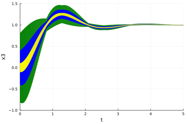
The task is to change the height from $0$ m to $1$ m within $5$ s. More precisely, a goal region $[0.98,1.02]$ of the height $x_3$ has to be reached within $5$ s and the height has to stay below $1.4$ m for all times. After $1$ s, the height should stay above $0.9$ m. The initial value for the position and velocities (i.e., from $x_1$ to $x_6$) is uncertain and given by $[-Δ, Δ]$ m, with $Δ = 0.4$. All other variables are initialized to $0$. This preliminary analysis must be followed by a corresponding evolution for $Δ = 0.1$ and $Δ = 0.8$ while keeping all the settings the same. No goals are specified for these cases: the objective instead is to understand the scalability of the tool.

const T = 5.0
const v3 = SingleEntryVector(3, 12, 1.0)

@inline function quad_property(sol)
    tf = tend(sol)

    # Condition: b1 = (x[3] < 1.4) for all time
    unsafe1 = HalfSpace(-v3, -1.4) # unsafe: -x3 <= -1.4
    b1 = all([isdisjoint(unsafe1, set(R)) for R in sol(0.0 .. tf)])
    #b1 = ρ(v3, sol) < 1.4

    # Condition: x[3] > 0.9 for t ≥ 1.0
    unsafe2 = HalfSpace(v3, 0.9) # unsafe: x3 <= 0.9
    b2 = all([isdisjoint(unsafe2, set(R)) for R in sol(1.0 .. tf)])

    # Condition: x[3] ⊆ Interval(0.98, 1.02) for t = 5.0
    b3 = set(project(sol[end]; vars=(3))) ⊆ Interval(0.98, 1.02)

    return b1 && b2 && b3
end

function quadrotor(; Wpos, Wvel)
    # initial condition
    ΔX0 = [Wpos, Wpos, Wpos, Wvel, Wvel, Wvel, 0.0, 0.0, 0.0, 0.0, 0.0, 0.0]
    X0 = Hyperrectangle(zeros(12), ΔX0)

    # initial-value problem
    prob = @ivp(x' = quadrotor!(x), dim:12, x(0) ∈ X0)

    return prob
end;

Analysis

Case 1: smaller uncertainty

Wpos = 0.1
Wvel = 0.1
prob = quadrotor(; Wpos=Wpos, Wvel=Wvel)
alg = TMJets(; abstol=1e-7, orderT=5, orderQ=1, adaptive=false)

sol = solve(prob; T=T, alg=alg)
solz1 = overapproximate(sol, Zonotope);

Verify that the specification holds:

@assert quad_property(solz1) "the property should be proven"

Case 2: intermediate uncertainty

Wpos = 0.4
Wvel = 0.4
prob = quadrotor(; Wpos=Wpos, Wvel=Wvel)
alg = TMJets(; abstol=1e-7, orderT=5, orderQ=1, adaptive=false)

sol = solve(prob; T=T, alg=alg)
solz2 = overapproximate(sol, Zonotope);

Verify that the specification holds:

@assert quad_property(solz2) "the property should be proven"

Case 3: large uncertainty

Wpos = 0.8
Wvel = 0.8
prob = quadrotor(; Wpos=Wpos, Wvel=Wvel)
alg = TMJets(; abstol=1e-7, orderT=5, orderQ=1, adaptive=false)

sol = solve(prob; T=T, alg=alg)
solz3 = overapproximate(sol, Zonotope);

The specification does not hold in this case:

@assert !quad_property(solz3) "the property should not be proven"

Results

using Plots

fig = plot(solz3; vars=(0, 3), linecolor="green", color=:green, alpha=0.8)
plot!(solz2; vars=(0, 3), linecolor="blue", color=:blue, alpha=0.8)
plot!(solz1; vars=(0, 3), linecolor="yellow", color=:yellow, alpha=0.8,
      xlab="t", ylab="x3",
      xtick=[0.0, 1.0, 2.0, 3.0, 4.0, 5.0], ytick=[-1.0, -0.5, 0.0, 0.5, 1.0, 1.5],
      xlims=(0.0, 5.0), ylims=(-1.0, 1.5))

References