Brusselator

Model description

A chemical reaction is said to be autocatalytic if one of the reaction products is also a catalyst for the same or a coupled reaction. We refer to Wikipedia for details.

The Brusselator is a mathematical model for a class of autocatalytic reactions. The dynamics of the Brusselator is given by the following two-dimensional differential equations.

\[\begin{aligned} \dot{x} &= A + x^2 ⋅ y - B ⋅ x - x \\ \dot{y} &= B ⋅ x - x^2 ⋅ y \end{aligned}\]

The numerical values for the model's constants (in their respective units) are $A = 1, B = 1.5$.

using ReachabilityAnalysis

@taylorize function brusselator!(du, u, p, t)
    local A = 1.0
    local B = 1.5
    local B1 = B + 1

    x, y = u

    x²y = x^2 * y
    du[1] = A + x²y - B1 * x
    du[2] = B * x - x²y
    return du
end

Specification

The initial set is $x ∈ [0.8, 1]$, $y ∈ [0, 0.2]$. The time horizon is $18$. These settings are taken from ^[CAS13].

U₀ = (0.8 .. 1.0) × (0.0 .. 0.2)
prob = @ivp(u' = brusselator!(u), u(0) ∈ U₀, dim:2)

T = 18.0;

Analysis

We use the TMJets algorithm with sixth-order expansion in time and second-order expansion in the spatial variables.

alg = TMJets21a(; orderT=6, orderQ=2)
sol = solve(prob; T=T, alg=alg);

Results

using Plots

fig = plot(sol; vars=(1, 2), xlab="x", ylab="y", lw=0.2, color=:blue,
           lab="Flowpipe", legend=:bottomright)
plot!(fig, U₀; color=:orange, lab="U₀")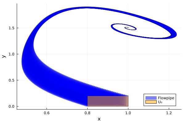

We observe that the system converges to the equilibrium point $(1.0, 1.5)$.

Below we plot the projected flowpipes over time.

fig = plot(sol; vars=(0, 1), xlab="t", lw=0.2, color=:blue, lab="x(t)", legend=:bottomright)
plot!(fig, sol; vars=(0, 2), lw=0.2, color=:red, lab="y(t)")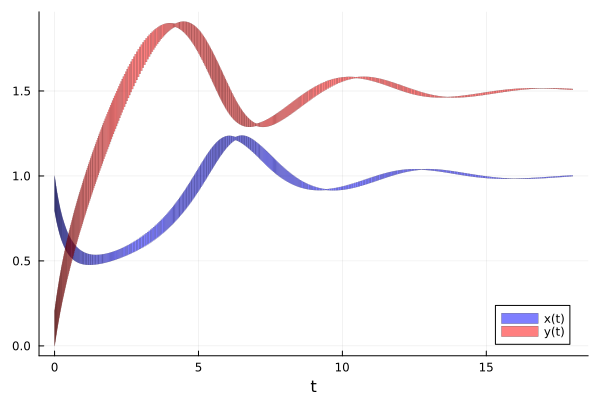

Changing the initial volume

The model was considered in ^[GCLISG20], but using a different set of initial states and a time horizon $30$. Let us parametrize the initial states as a square centered at $x = y = 1$ and radius $r > 0$:

U0(r) = BallInf([1.0, 1.0], r);

The parametric initial-value problem is defined accordingly.

bruss(r) = @ivp(u' = brusselator!(u), u(0) ∈ U0(r), dim:2);

First we solve for $r = 0.01$:

sol_01 = solve(bruss(0.01); T=30.0, alg=alg);

old_ztol = LazySets._ztol(Float64)
LazySets.set_ztol(Float64, 1e-15)  # use higher precision for the plots

fig = plot(sol_01; vars=(1, 2), xlab="x", ylab="y", lw=0.2, color=:blue, lab="Flowpipe (r = 0.01)",
           legend=:bottomright)
plot!(fig, U0(0.01); color=:orange, lab="Uo", xlims=(0.6, 1.3))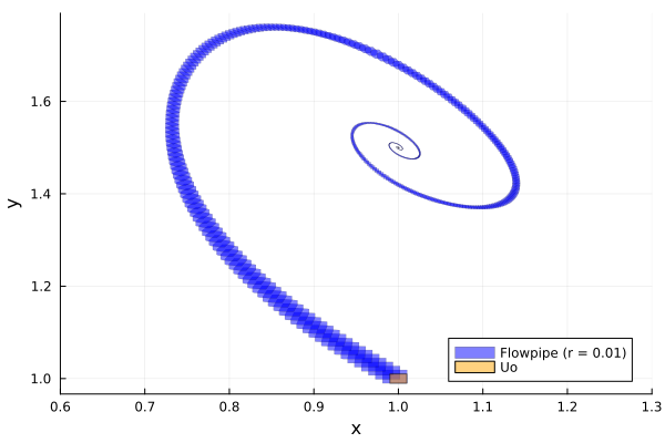

We observe that the wrapping effect is controlled and the flowpipe does not blow up even for the large time horizon $T = 30.0$. Next we plot the flowpipe zoomed to the last portion and compare $r = 0.01$ with a larger set of initial states, $r = 0.1$.

sol_1 = solve(bruss(0.1); T=30.0, alg=alg);

fig = plot(; xlab="x", ylab="y", xlims=(0.9, 1.05), ylims=(1.43, 1.57), legend=:bottomright)
plot!(fig, sol_1; vars=(1, 2), lw=0.2, color=:red, lab="r = 0.1", alpha=0.4)
plot!(fig, sol_01; vars=(1, 2), lw=0.2, color=:blue, lab="r = 0.01")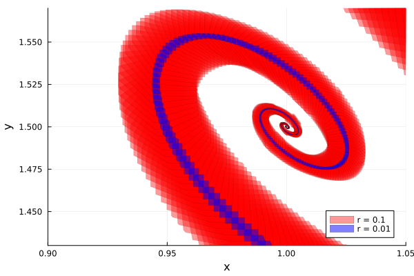

LazySets.set_ztol(Float64, old_ztol);  # reset precision

The volume at time $T = 9.0$ can be (over)estimated by evaluating the flowpipe and computing the volume of a hyperrectangular overapproximation:

vol_01 = volume(set(overapproximate(sol_01(9.0), Hyperrectangle)))

1.7055195351344024e-5

vol_1 = volume(set(overapproximate(sol_1(9.0), Hyperrectangle)))

0.0009160016041017206

References