International Space Station

Model description

This is a model of component 1r (Russian service module) of the International Space Station ^[ASG00]. It has 270 states, 3 inputs and 3 outputs. The model consists of a continuous linear time-invariant system

\[\begin{aligned} \dot{x}(t) &= Ax(t) + Bu(t),\qquad u(t) ∈ \mathcal{U} \\ y(t) &= Cx(t) \end{aligned}\]

It was proposed as a benchmark in ARCH 2016 ^[TLT16]. The matrix dimensions are $A ∈ \mathbb{R}^{270 × 270}$, $B ∈ \mathbb{R}^{270 × 3}$, and $C ∈ \mathbb{R}^{3 × 270}$.

The matrices A, B, and C are available in MATLAB format here (iss.mat). For convenience, the .mat file has been converted to the JLD2 format and stored in iss.jld2.

There are two versions of this benchmark, ISSF01 (time-varying inputs) and ISSC01 (constant inputs).

• ISSF01 (time-varying inputs): In this setting, the inputs can change arbitrarily over time: $\forall t: u(t) ∈ \mathcal{U}$.

• ISSC01 (constant inputs): The inputs are only uncertain in their initial value, and constant over time: $u(0) ∈ \mathcal{U}$, $\dot{u}(t) = 0$.

using ReachabilityAnalysis, JLD2, ReachabilityBase.CurrentPath
using ReachabilityAnalysis: add_dimension

path = @current_path("ISS", "ISS.jld2")

@load path C
const C3 = C[3, :]  # variable y₃
const C3_ext = vcat(C3, fill(0.0, 3));

Specifications

Initially, all variables are in the range $[-0.0001, 0.0001]$, and the inputs are bounded: $u_1(t) ∈ [0, 0.1]$, $u_2(t) ∈ [0.8, 1]$, and $u_3(t) ∈ [0.9, 1]$. The time bound is $20$.

The verification goal is to check the ranges reachable by the output $y_3(t)$, which is a linear combination of the state variables. In addition to the safety specification, for each version there is an UNSAT instance that serves as sanity checks to ensure that the model and the tool work as intended. But there is a caveat: In principle, verifying an UNSAT instance only makes sense formally if a witness is provided (counterexample, underapproximation, etc.). We instead run the tool with the same accuracy settings on an SAT-UNSAT pair of instances. The SAT instance demonstrates that the overapproximation is not too coarse, and the UNSAT instance demonstrates that the overapproximation is indeed conservative.

• ISS01: Bounded time, safe property: For all $t ∈ [0, 20]$, $y_3(t) ∈ [−0.0007, 0.0007]$. This property is used with the uncertain input case (ISSF01) and should be proven.

• ISS02: Bounded time, safe property: For all $t ∈ [0, 20]$, $y_3(t) ∈ [−0.0005, 0.0005]$. This property is used with the constant input case (ISSC01) and should be proven.

• ISU01: Bounded time, unsafe property: For all $t ∈ [0, 20]$, $y_3 (t) ∈ [−0.0005, 0.0005]$. This property is used with the uncertain input case (ISSF01) and should not be proven.

• ISU02: Bounded time, unsafe property: For all $t ∈ [0, 20]$, $y_3 (t) ∈ [−0.00017, 0.00017]$. This property is used with the constant input case (ISSC01) and should not be proven.

function ISS_common(n)
    X0 = BallInf(zeros(n), 0.0001)
    U = Hyperrectangle(; low=[0.0, 0.8, 0.9], high=[0.1, 1.0, 1.0])
    return X0, U
end

function ISSF01()
    @load path A B
    X0, U = ISS_common(size(A, 1))
    return @ivp(x' = A * x + B * u, x(0) ∈ X0, u ∈ U, x ∈ Universe(270))
end

function ISSC01()
    @load path A B
    A_ext = add_dimension(A, 3)
    A_ext[1:270, 271:273] = B
    X0, U = ISS_common(size(A, 1))
    return @ivp(x' = A_ext * x, x(0) ∈ X0 * U)
end;

Results

The specification involves only the output $y(t) := C_3 x(t)$, where $C_3$ denotes the third row of the output matrix $C ∈ \mathbb{R}^{3 × 270}$. Hence, it is sufficient to compute the flowpipe associated with $y(t)$ directly, without the need of actually computing the full 270-dimensional flowpipe associated with all state variables. The flowpipe associated with a linear combination of state variables can be computed efficiently using the support-function based algorithm [LGG09]. The idea is to define a template polyhedron with only two supporting directions, namely $C_3$ and $-C_3$.

The chosen step sizes are $6×10^{-4}$ for ISSF01 and $1×10^{-2}$ for ISSC01.

ISSF01

dirs = CustomDirections([C3, -C3])
prob_ISSF01 = ISSF01()
sol_ISSF01 = solve(prob_ISSF01; T=20.0,
                   alg=LGG09(; δ=6e-4, template=dirs, sparse=true, cache=false));

The solution sol_ISSF01 is a 270-dimensional set that (only) contains template reach sets for the linear combination C_3 x(t).

dim(sol_ISSF01)

270

For visualization, it is necessary to specify that we want to plot "time" vs. $y_3(t)$. We can transform the flowpipe on the output $y_3(t)$ by "flattening" the flowpipe along directions dirs.

πsol_ISSF01 = flatten(sol_ISSF01);

Now πsol_ISSF01 is a one-dimensional flowpipe.

dim(πsol_ISSF01)

1

using Plots, Plots.PlotMeasures, LaTeXStrings

old_ztol = LazySets._ztol(Float64)
LazySets.set_ztol(Float64, 1e-8);  # use higher precision for the plots

fig = plot(πsol_ISSF01[1:10:end]; vars=(0, 1), linecolor=:blue, color=:blue,
           alpha=0.8, xlab=L"t", ylab=L"y_{3}", xtick=[0, 5, 10, 15, 20.0],
           ytick=[-0.00075, -0.0005, -0.00025, 0, 0.00025, 0.0005, 0.00075],
           xlims=(0.0, 20.0), ylims=(-0.00075, 0.00075),
           bottom_margin=6mm, left_margin=2mm, right_margin=4mm, top_margin=3mm)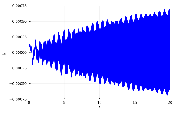

ISSC01

dirs = CustomDirections([C3_ext, -C3_ext])
prob_ISSC01 = ISSC01()
sol_ISSC01 = solve(prob_ISSC01; T=20.0,
                   alg=LGG09(; δ=0.01, template=dirs, sparse=true, cache=false));

We can flatten the flowpipe to the output $y_3(t)$ as before:

πsol_ISSC01 = flatten(sol_ISSC01);

fig = plot(πsol_ISSC01; vars=(0, 1), linecolor=:blue, color=:blue, alpha=0.8,
           lw=1.0, xlab=L"t", ylab=L"y_{3}", xtick=[0, 5, 10, 15, 20.0],
           ytick=[-0.0002, -0.0001, 0.0, 0.0001, 0.0002],
           xlims=(0.0, 20.0), ylims=(-0.0002, 0.0002),
           bottom_margin=6mm, left_margin=2mm, right_margin=4mm, top_margin=3mm)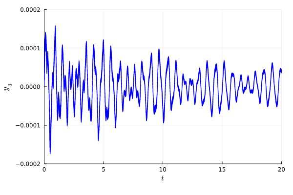

LazySets.set_ztol(Float64, old_ztol);  # reset precision

References