Laub-Loomis

Model description

The Laub-Loomis model is presented in ^[LL98] for studying a class of enzymatic activities. The dynamics can be defined by the following seven-dimensional system of differential equations.

using ReachabilityAnalysis

@taylorize function laubloomis!(dx, x, p, t)
    dx[1] = 1.4 * x[3] - 0.9 * x[1]
    dx[2] = 2.5 * x[5] - 1.5 * x[2]
    dx[3] = 0.6 * x[7] - 0.8 * (x[2] * x[3])
    dx[4] = 2 - 1.3 * (x[3] * x[4])
    dx[5] = 0.7 * x[1] - (x[4] * x[5])
    dx[6] = 0.3 * x[1] - 3.1 * x[6]
    dx[7] = 1.8 * x[6] - 1.6 * (x[2] * x[7])
    return dx
end

The system is asymptotically stable and the equilibrium is the origin.

Specification

The initial conditions are defined according to the ones used in ^[TD13]. They are boxes centered at $x_1(0) = 1.2$, $x_2(0) = 1.05$, $x_3(0) = 1.5$, $x_4(0) = 2.4$, $x_5(0) = 1$, $x_6(0) = 0.1$, $x_7 (0) = 0.45$. The range of the box in the i-th dimension is defined by the interval $[x_i(0) − W, x_i(0) + W]$. We consider $W = 0.01$, $W = 0.05$, and $W = 0.1$. The specification for each scenario is given as follows:

• $W = 0.01$ and $W = 0.05$: The unsafe region is defined by $x_4 ≥ 4.5$.
• $W = 0.1$: The unsafe set is defined by $x_4 ≥ 5$.

The time horizon for all cases is $[0, 20]$.

function laubloomis(; W=0.01)
    X0 = Hyperrectangle([1.2, 1.05, 1.5, 2.4, 1.0, 0.1, 0.45], fill(W, 7))
    prob = @ivp(x' = laubloomis!(x), dim:7, x(0) ∈ X0)
    return prob
end;

Analysis

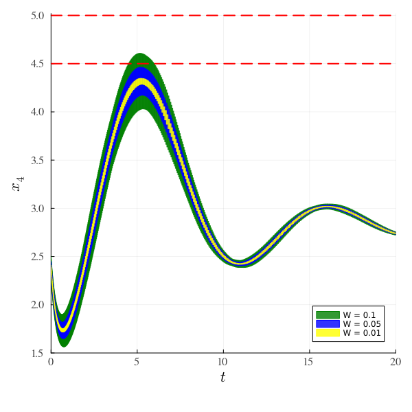
The final widths of $x_4$ along with the computation times are computed for all three cases, as well as a figure in the $(t, x_4)$ axes, with $t ∈ [0, 20]$, $x_4 ∈ [1.5, 5]$, where the three plots are overlaid.

Canonical direction along x₄:

const e4 = [0.0, 0.0, 0.0, 1.0, 0.0, 0.0, 0.0];

Case 1: Small initial set

In this case, we consider the width of the initial set $W = 0.01$.

prob = laubloomis(; W=0.01)
alg = TMJets(; abstol=1e-11, orderT=7, orderQ=1, adaptive=true)

sol_1 = solve(prob; T=20.0, alg=alg)
sol_1z = overapproximate(sol_1, Zonotope);

We verify that the specification holds:

@assert ρ(e4, sol_1z) < 4.5 "the property should be proven"
ρ(e4, sol_1z)

4.347181052143644

To compute the width of the final box, we use the support function:

ρ(e4, sol_1z[end]) + ρ(-e4, sol_1z[end])

0.004238950465202507

Case 2: Intermediate initial set

In this case, we consider the width of the initial set $W = 0.05$.

prob = laubloomis(; W=0.05)
alg = TMJets(; abstol=1e-12, orderT=7, orderQ=1, adaptive=false)

sol_2 = solve(prob; T=20.0, alg=alg)
sol_2z = overapproximate(sol_2, Zonotope);

We verify that the specification holds:

@assert ρ(e4, sol_2z) < 4.5 "the property should be proven"
ρ(e4, sol_2z)

4.462157651009224

Width of final box:

ρ(e4, sol_2z[end]) + ρ(-e4, sol_2z[end])

0.017468964603667203

Case 3: Large initial set

In this case, we consider the width of the initial set $W = 0.1$.

prob = laubloomis(; W=0.1)
alg = TMJets(; abstol=1e-12, orderT=7, orderQ=1, adaptive=false)

sol_3 = solve(prob; T=20.0, alg=alg)
sol_3z = overapproximate(sol_3, Zonotope);

We verify that the specification holds:

@assert ρ(e4, sol_3z) < 5.0 "the property should be proven"
ρ(e4, sol_3z)

4.607152446545931

Width of final box:

ρ(e4, sol_3z[end]) + ρ(-e4, sol_3z[end])

0.03370610732515722

Results

using Plots, Plots.PlotMeasures, LaTeXStrings

fig = plot(sol_3z; vars=(0, 4), linecolor="green", color=:green, alpha=0.8, lab="W = 0.1")
plot!(fig, sol_2z; vars=(0, 4), linecolor="blue", color=:blue, alpha=0.8, lab="W = 0.05")
plot!(fig, sol_1z; vars=(0, 4), linecolor="yellow", color=:yellow, alpha=0.8, lab="W = 0.01",
      tickfont=font(10, "Times"), guidefontsize=15, xlab=L"t", ylab=L"x_4",
      xtick=[0.0, 5.0, 10.0, 15.0, 20.0], ytick=[1.5, 2.0, 2.5, 3.0, 3.5, 4.0, 4.5, 5.0],
      xlims=(0.0, 20.0), ylims=(1.5, 5.02),
      bottom_margin=6mm, left_margin=2mm, right_margin=4mm, top_margin=3mm,
      size=(600, 600))
plot!(fig, x -> x, x -> 4.5, 0.0, 20.0; line=2, color="red", linestyle=:dash, lab="")
plot!(fig, x -> x, x -> 5.0, 0.0, 20.0; line=2, color="red", linestyle=:dash, lab="")

References