Frequently Asked Questions (FAQ)

General questions

What are good introductory papers on the subject?

An elementary introduction to the principles of set-based numerical integration can be found in Oded Maler's article Computing Reachable Sets: An Introduction. For an introduction to hybrid systems reachability we recommend the lecture notes of Prof. Goran Frehse, Formal Verification of Piecewise Affine Hybrid Systems (DigiCosme Spring School, Paris, May 2016). Most up-to-date material related to reachability analysis can be found in journals, conference articles or in PhD theses. For a comprehensive review of different set propagation techniques for linear, nonlinear and hybrid systems see [AFG20]. The article also contains a discussion of successful applications of reachability analysis to real-world problems. We refer to the References section of this manual for further links to the relevant literature.

Are there other tools that perform reachability analysis?

The wiki Related Tools contains an extensive list of pointers related to reachability analysis tools for dynamical systems. Languages and tools for hybrid systems design are described in the review article [CPPSV06] (a bit outdated with respect to the tools since it is of 2006).

A subset of such tools has participated in recent editions of the Friendly Competition for Applied Reachability of Continuous and Hybrid Systems, ARCH-COMP. In alphabetic order: Ariadne, CORA, C2E2, DynIbex, Flow*, HyDRA, Hylaa, Isabelle/HOL-ODE-Numerics, SpaceEx and XSpeed. A paragraph describing each tool's main characteristics can be found in the ARCH-COMP articles for each category (AFF for linear and NLN for nonlinear).

The IEEE Control Systems Society (CSS) has a Technical Committee on Hybrid Systems that is dedicated to providing informational forums, meetings for technical discussion, and information over the web to researchers in the IEEE CSS who are interested in the field of hybrid systems and its applications. A list of actively-maintained tools for the analysis and synthesis of hybrid systems, compiled by members of such committee, can be found here.

Why did you choose Julia to write this library?

The language choice when programming for research purposes usually depends on the developers' background knowledge which directly impacts convenience during development and output performance in the final product. On the one hand, compiled languages such as C++ offer high performance, but the compilation overhead is inconvenient for prototyping. On the other hand, interpreted languages such as Python offer an interactive session for convenient prototyping, but these languages fall behind in performance or need to extend the code to work with another lower-layer program such as Numba or Cython (known as the two-language problem). A compromise between the two worlds are just-in-time (JIT) compiled languages such as MATLAB. Last but not least, the ecosystem of libraries available and the user base is also an important consideration.

In our case, we began to develop the JuliaReach stack in 2017 and quickly adopted the language when it was at its v0.5 ^[v1]. Julia is a general-purpose programming language but it was conceived with high-performance scientific computing in mind, and it reconciles the two advantages of compiled and interpreted languages described above, as it comes with an interactive read-evaluate-print loop (REPL) front-end, but is JIT compiled to achieve performance that is competitive with compiled languages such as C ^[BEKS17]. A distinctive feature of Julia is multiple dispatch (i.e., the function to execute is chosen based on each argument type), which allows to write efficient machine code based on a given type, e.g., of the set. As additional features, Julia is platform independent, has an efficient interface to C and FORTRAN, is supported in Jupyter notebooks (the "Ju" in Jupyter is for Julia) and well-suited for parallel computing. Julia has a determined and quickly-growing community, especially for scientific tools (see the JuliaLang Community webpage). All this makes Julia an interesting programming language for writing a library for reachability analysis.

What is the wrapping effect?

Quoting a famous paper by R. E. Moore [M65]:

Under the flow itself a box is carried after certain time into a set of points which will in general not remain a box excepted for a few simple flows.

The wrapping effect is associated to error propagation that arises from the inability of a set representation to accurately abstract some properties of system under study. Wrapping-free methods only exist for linear systems. Nonlinear reachability methods control, but do not totally elimitate, the wrapping effect in different ways.

As a simple illustration of the wrapping effect, consider the image of a box through a rotation in discrete time-steps. Box enclosures (full line) introduce a strong wrapping effect. On the other hand, had we represented the sequence using zonotopes (dashed lines), the result would be exact, i.e. without wrapping, since the image of a hyperrectangular set under an affine map is a zonotope.

using LazySets, Plots

R(θ) = [cos(θ) -sin(θ); sin(θ) cos(θ)]

B = BallInf(ones(2), 0.1)
B′ = R(π/4) * B
B′′ = R(π/2) * B

□B = box_approximation(B)
□B′ = box_approximation(B′)
□B′′ = box_approximation(R(π/4) * □B′)

fig = plot(B, ratio=1, lw=2.0, style=:dash)
plot!(B′, lw=2.0, style=:dash)
plot!(B′′, lw=2.0, style=:dash)

plot!(□B, lw=2.0, style=:solid)
plot!(□B′, lw=2.0, style=:solid)
plot!(□B′′, lw=2.0, style=:solid)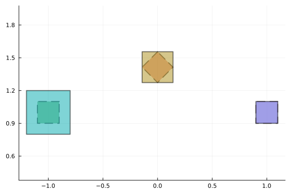

Does reachability solve for the vertices of the set?

What happens if you consider a chaotic system?

Can reachability analysis be used to solve large problems?

Solving capabilities

How can I visualize trajectories?

It is often necessary to plot a "bunch" of trajectories starting from a set of initial conditions. The parallel ensemble simulations capabilities from the Julia OrdinaryDiffEq.jl suite can be used to numerically simulate a given number of trajectories and it counts with state-of-the-art algorithms for stiff and non-stiff ODEs as well as many other advanced features, such as distributed computing, multi-threading and GPU support. See EnsembleAlgorithms for details.

As a simple example consider the scalar ODE $x'(t) = 1.01x(t)$ with initial condition on the interval $x(0) ∈ [0, 0.5]$. To solve it using ensemble simulations, pass the ensemble=true keyword argument to the solve function (if the library OrdinaryDiffEq was not loaded in your current session, an error is triggered). The number of trajectories can be specified with the trajectories keyword argument.

using ReachabilityAnalysis, OrdinaryDiffEq

# formulate initial-value problem
prob = @ivp(x' = 1.01x, x(0) ∈ 0 .. 0.5)

# solve the flowpipe using a default algorithm, and also compute trajectories
sol = solve(prob, tspan=(0.0, 1.0), ensemble=true, trajectories=250)

# plot flowpipe and the ensemble solution
using Plots

fig = plot(sol, vars=(0, 1), linewidth=0.2, xlab="t", ylab="x(t)")
plot!(ensemble(sol), vars=(0, 1), linealpha=1.0)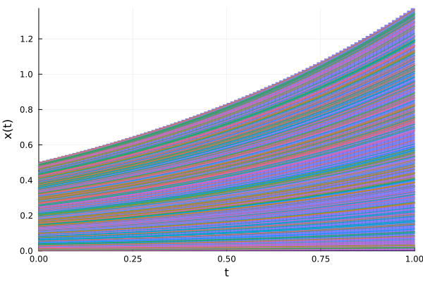

Please note that the latency (compilation time) of the first using line is long, typically one minute with Julia v1.5.3.

Can I solve a for a single initial condition?

To solve for a single initial condition, i.e. a "point", use Singleton as the initial set (singleton means a set with one element). For example, here we plot the free vibration solution of a standard single degree of freedom system without physical damping,

\[ x''(t) + 4x(t) = 0, \qquad x(0) = 1,\qquad x'(0) = 0.\]

In this initial-value problem, the initial condition is given as a point that we can model as X0 = Singleton([1.0, 0.0]), where we associate the first coordinate to position, x(t), and the second coordinate to velocity, x'(t).

Below we plot the flowpipe for the same initial condition and different step sizes.

using ReachabilityAnalysis, Plots

# x' = v
# v' = -4x
A = [0 1; -4. 0]
X0 = Singleton([1.0, 0.0])
prob = @ivp(X' = AX, X(0) ∈ X0)

f(ΔT) = solve(prob, tspan=(0.0, 5.0), alg=GLGM06(δ=ΔT))

fig = plot(f(0.3), vars=(0, 1), lab="ΔT=0.3", color=:yellow)
plot!(f(0.1), vars=(0, 1), lab="ΔT=0.1", color=:lightblue)
plot!(f(0.05), vars=(0, 1), xlab="time", ylab="x(t)", lab="ΔT=0.05", color=:green)

dom = 0:0.01:5.0
plot!(dom, cos.(2.0 * dom), lab="Analytic", color=:magenta)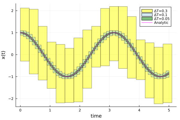

Why do I see boxes for single initial conditions?

As it is seen in the question Can I solve a for a single initial condition?, even if the initial condition is a singleton, the obtained flowpipe is a sequence of boxes in the x-t plane, i.e. we obtain sets with non-zero width both in time and in space. This behavior may seem confusing at first, because the initial conditions where deterministic. The catch is that reach-sets represents a set of states reachable over a time interval, that certainly contains the exact solution for the time-span associated to the reach-set, tspan(R). The projection of the flowpipe on the time axis thus returns a sequence of intervals, their width being the step size of the method (in case the method has fixed step size). When we take the Cartesian product of each time span with the projection of the flowpipe in x(t), we obtain a box.

If we consider two different step-sizes, the area of the boxes shrinks. It is known theoretically that the flowpipe converges, in Hausdorff norm, to the exact flowpipe. The plot below illustrates the convergence for aspects for two different step sizes, ΔT=0.1 and ΔT=0.05, evaluating the solution around the time point 3.0. The projection onto x(t) (vertical axis) shows that dividing the step size by half, we can more accurately know the exact value of the solution, and the width of the boxes intersecting the time point 3.0 decrease by a factor 2.5x.

fig = plot(f(0.1)(3.0), vars=(0, 1), xlab="time", ylab="x(t)", lab="ΔT=0.1", color=:lightblue)

I(Δt, t) = -ρ([-1.0, 0.0], f(Δt)(t)) .. ρ([1.0, 0.0], f(Δt)(t)) |> Interval

I01 = I(0.1, 3.0)
plot!(y -> max(I01), xlims=(2.9, 3.1), lw=3.0, style=:dash, color=:lightblue, lab="Δx = $(I01.dat)")
plot!(y -> min(I01), xlims=(2.9, 3.1), lw=3.0, style=:dash, color=:lightblue, lab="")
plot!(f(0.05)(3.0), vars=(0, 1), xlab="time", ylab="x(t)", lab="ΔT=0.05", color=:green)

I005 = I(0.05, 3.0)
plot!(y -> max(I005), xlims=(2.9, 3.1), lw=3.0, style=:dash, color=:green, lab="Δx = $(I005.dat)")
plot!(y -> min(I005), xlims=(2.9, 3.1), lw=3.0, style=:dash, color=:green, lab="")

dom = 2.9:0.01:3.1
plot!(dom, cos.(2.0 * dom), lab="Analytic", color=:magenta, legend=:bottomright)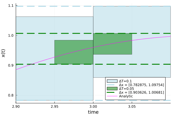

Why do some trajectories escape the flowpipe?

Can I compute solutions using parallel programming?

Yes. You can compute multiple flowpipes in parallel by defining an initial-value problem with an array of initial conditions. This methods uses Julia's multithreaded parallelism, so you have to set the number of threads to use before starting Julia. The following example illustrates this point. For further details we refer to the section Distributed computations.

using ReachabilityAnalysis, Plots

A = [0.0 1.0; -1.0 0.0]

B = [BallInf([0,0.] .+ k, 0.1) for k in 1:5]
prob = @ivp(x' = Ax, x(0) ∈ B)

# multi-threaded solve
sol = solve(prob, T=12.0, alg=GLGM06(δ=0.02));
fig = plot(sol, vars=(0, 2), c=:red, alpha=.5, lw=0.2, xlab="t", ylab="y")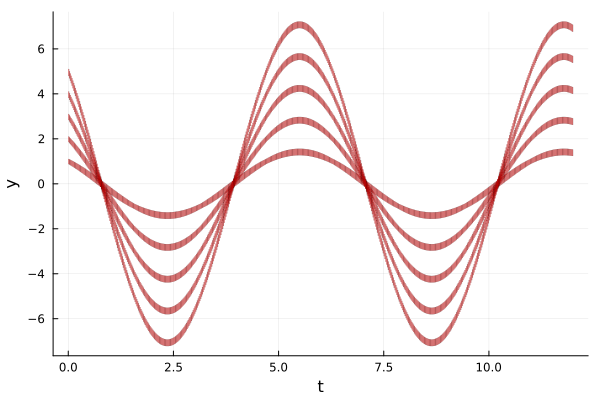

On the other hand, please note that in the example of above, you can compute with a single integration the flowpipe corresponding to the convex hull of the elements in the array B.

prob = @ivp(x' = Ax, x(0) ∈ ConvexHullArray(B))
sol = solve(prob, T=12.0, alg=GLGM06(δ=0.02, approx_model=Forward()));
plot!(sol, vars=(0, 2), c=:lightgreen, alpha=.5, lw=0.2, xlab="t", ylab="y")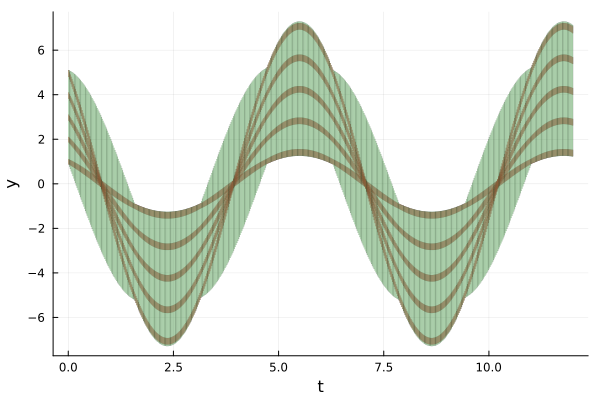

Modeling questions

Can I use ODE solvers with interval initial conditions?

Although it is in principle possible to ODE solvers for

How do I use the @taylorize macro?

The section Some common gotchas of the user manual details do's and dont's for the @taylorize macro to speedup reachability computations using Taylor models.

A note on interval types

When using intervals as set representation, ReachabilityAnalysis.jl relies on rigorous floating-point arithmetic implemented in pure Julia in the library IntervalArithmetic.jl (we often use const IA = IntervalArithmetic as an abbreviation). The main struct defined in the library is IA.Interval (and the corresponding multi-dimensional interval is IA.IntervalBox). Internally, the set LazySets.Interval is wrapper-type of IA.Interval and these two types should not be confused, although our user APIs extensively use duck typing, in the sense that x(0) ∈ 0 .. 1 (IA.Interval type) and x(0) ∈ Interval(0, 1) are valid.

On a technical level, the reason to have LazySets.Interval as a wrapper type of IA.Interval is that Julia doesn't allow multiple inheritance, but it was a design choice that intervals should belong to the LazySets type hierarchy.

References

- v1Version 1.0 of the language was released in August 2018; see this blog post.