Lotka-Volterra

Model description

The 2-dimensional Lotka-Volterra system depicts the population change of a class of predators and a class of preys. The growth rate of the prey population $x$ over time is governed by the differential equation

\[ \dot{x} = α x - β x y,\]

where $α$, $β$ are constant parameters and $y$ is the population of predators. We can see that the number of prey grows exponentially without predation.

The population growth of predators is governed by the differential equation

\[ \dot{y} = δ x y - γ y,\]

where $γ, δ$ are constant parameters.

We set these parameters to $α = 1.5$, $β = 1$, $γ = 3$, and $δ = 1$.

using ReachabilityAnalysis

@taylorize function lotkavolterra!(du, u, p, t)
    local α, β, γ, δ = 1.5, 1.0, 3.0, 1.0

    x, y = u
    xy = x * y
    du[1] = α * x - β * xy
    du[2] = δ * xy - γ * y
    return du
end

Specification

We consider the initial set $x ∈ [4.8, 5.2], y ∈ [1.8, 2.2]$.

X0 = Hyperrectangle(; low=[4.8, 1.8], high=[5.2, 2.2])
prob = @ivp(x' = lotkavolterra!(x), dim:2, x(0) ∈ X0);

Analysis

sol = solve(prob; T=8.0, alg=TMJets())
solz = overapproximate(sol, Zonotope);

Results

using Plots

fig = plot(solz; vars=(1, 2), alpha=0.3, lw=0.0, xlab="x", ylab="y",
           lab="Flowpipe", legend=:bottomright)
plot!(fig, X0; label="X(0)")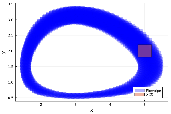

Adding parameter variation

In this setting, we consider all parameters as uncertain model constants. In addition, we add another term $ϵ$ to the first differential equation.

@taylorize function lotkavolterra_parametric!(du, u, p, t)
    x, y, αp, βp, γp, δp, ϵp = u
    xy = x * y
    du[1] = αp * x - βp * xy - ϵp * x^2
    du[2] = δp * xy - γp * y

    # encode uncertain parameters
    du[3] = zero(αp)
    du[4] = zero(βp)
    du[5] = zero(γp)
    du[6] = zero(δp)
    du[7] = zero(ϵp)
    return du
end

Specification

p_int = (0.99 .. 1.01) × (0.99 .. 1.01) × (2.99 .. 3.01) × (0.99 .. 1.01) × (0.099 .. 0.101)
U0 = cartesian_product(Singleton([1.0, 1.0]), convert(Hyperrectangle, p_int))
prob = @ivp(u' = lotkavolterra_parametric!(u), dim:7, u(0) ∈ U0);

Analysis

sol = solve(prob; tspan=(0.0, 10.0))
solz = overapproximate(sol, Zonotope);

Results

fig = plot(solz; vars=(1, 2), lw=0.3, title="Uncertain parameters",
           lab="abstol = 1e-15", xlab="x", ylab="y")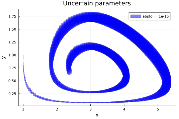

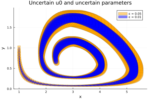
Uncertain initial condition (u0)

Now we consider an initial box around u0

$ϵ = 0.05$

In this setting, we consider the uncertain parameter $ϵ$ with radius $0.05$.

Specification

□(ϵ) = BallInf([1.0, 1.0], ϵ)

U0 = cartesian_product(□(0.05), convert(Hyperrectangle, p_int))
prob = @ivp(u' = lotkavolterra_parametric!(u), dim:7, u(0) ∈ U0);

Analysis

sol = solve(prob; T=10.0, alg=TMJets(; abstol=1e-10))
solz = overapproximate(sol, Zonotope);

Results

fig = plot(solz; vars=(1, 2), color=:orange, lw=0.3, lab="ϵ = 0.05",
           title="Uncertain u0 and uncertain parameters", xlab="x", ylab="y")

$ϵ = 0.01$

In this setting, we consider the uncertain parameter $ϵ$ with radius $0.01$.

Specification

U0 = cartesian_product(□(0.01), convert(Hyperrectangle, p_int))
prob = @ivp(u' = lotkavolterra_parametric!(u), dim:7, u(0) ∈ U0);

Analysis

sol = solve(prob; T=10.0, alg=TMJets(; abstol=1e-10))
solz = overapproximate(sol, Zonotope);

Results

plot!(solz; vars=(1, 2), color=:blue, lw=0.3, lab="ϵ = 0.01")