Transmission line circuit
System type: Linear continuous system
State dimension: parametric, typically between 4 to 40
Application domain: Power systems stability
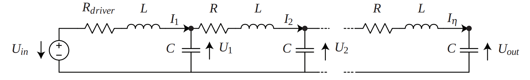
We consider the transmission line model used in Althoff et al. [AKS11]. The RLC circuit of the transmission line is shown below. In the circuit, $U_{in}$ is the voltage at the sending end, and $U_{out}$ is the voltage at the receiving end.
Model description
For reference to understand this model, we refer to standard textbooks on electrical circuits. The electrical elements law for resistors (R), inductors (L), and capacitors (C) are studied, for instance, in Kluever [Klu20], Chapter 3.
Let's assume that the circuit consists of $η > 2$ nodes. There are $η$ dynamic equations for the capacitor voltages and $η$ dynamic equations for the circuit currents. Therefore, the state vector can be represented as
\[ x = [U_1, U_2, …, U_η, I_1, I_2, …, I_η]^T,\]
and the state dimension is $2η$.
Analysis of the first node
When writing the equations for the voltages and currents, we should pay attention to the sign choices in the given circuit, which do not exactly match the convention in text books (in the sense that the $U_1$s positive terminal is at the bottom, as indicated by the arrows). Let $R_d$ denote the driver resistance's current. By Kirchhoff's voltage law,
\[ U_{in} = R_d I_1 + LI_1' - U_1.\]
Therefore,
\[ \boxed{I_1' = \dfrac{U_{in} + U_1}{L} - \dfrac{R_d}{L}I_1}.\]
By Kirchhoff's current law, and if $I_{1, C}$ denotes the current through the capacitor $C$, connected to the first node,
\[ I_1 = I_2 + I_{C, 1},\]
and
\[I_{C, 1} = -CU_1'.\]
Hence
\[ \boxed{U_1' = \dfrac{I_2 - I_1}{C}}.\]
Analysis of the intermediate nodes
The intermediate nodes' equations are obtained in a similar fashion. For instance, for the second loop one has
\[ -U_1 = RI_2 + LI_2' - U_2 ⇒ I_2' = \dfrac{U_2-U_1}{L} - \dfrac{R}{L}I_2\]
for the current's equation, and
\[ I_{2, C} = I_2 - I_3 ⇒ U_2' = \dfrac{I_3 - I_2}{C}.\]
for the voltage's equation.
Generalizing to arbitrary $l = 2, \ldots, η - 1$ is trivial and gives:
\[ \boxed{I'_l = \dfrac{U_l - U_{l-1}}{L} - \dfrac{R}{L}I_l} \\ \boxed{U'_l = \dfrac{I_{l+1} - I_l}{C}}.\]
Analysis of the last node
The last node corresponds to the case $l = η$.
\[ \boxed{I'_η = \dfrac{U_η - U_{η-1}}{L} - \dfrac{R}{L}I_η}, \\ \boxed{U'_{out} = U'_{out} = - \dfrac{I_{η}}{C}}.\]
System of linear differential equations
Recall that the stateset is $\mathbb{R}^{2η}$, where the state variables are $x = [U_1, U_2, \ldots, U_η, I_1, I_2, \ldots, I_η]^T$. The system can be written as a block-diagonal system of linear differential equations,
\[ x'(t) = Ax(t) + BU_{in}(t),\]
using the results in the previous section.
The coefficients matrix $A$ can be written as a block-diagonal matrix. There are useful constructors in the base package LinearAlgebra that greatly simplify building matrices with special shape, as in our case, such as diagonal and band matrices, with the types Diagonal and Bidiagonal.
We consider the case of $η = 20$ nodes as in Althoff et al. [AKS11], such that the system has $n = 40$ state variables.
using ReachabilityAnalysis, LinearAlgebra, SparseArrays

function tline(; η=3, R=1.00, Rd=10.0, L=1e-10, C=1e-13 * 4.00)
    A₁₁ = zeros(η, η)
    A₁₂ = Bidiagonal(fill(-1 / C, η), fill(1 / C, η - 1), :U)
    A₂₁ = Bidiagonal(fill(1 / L, η), fill(-1 / L, η - 1), :L)
    A₂₂ = Diagonal(vcat(-Rd / L, fill(-R / L, η - 1)))
    A = [A₁₁ A₁₂; A₂₁ A₂₂]
    B = sparse([η + 1], [1], 1 / L, 2η, 1)
    return A, B
end

η = 20
n = 2η
A, B = tline(; η=η);
We can visualize the structure of the sparse coefficients matrix $A$ for the case $η = 20$ with a spy plot:
using Plots

fig = spy(A; legend=nothing, markersize=2.0, title="Sparsity pattern of A",
          xlab="columns", ylab="rows")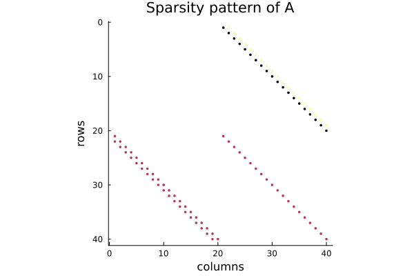
Notice that the matrix coefficients are rather large. Hence it is convenient to rescale the system for numerical stability. Let $α > 0$ be a scaling factor, and let $\tilde{x}(t) = x(α t)$. By the chain rule,
\[ \tilde{x}'(t) = α x'(α t) = α A x(α t) + α B U_{in}(α t) = \tilde{A} \tilde{x}(t) + \tilde{B} \tilde{U}_{in}(t),\]
where $\tilde{A} := α A$ and $\tilde{B} := α B$.
function scale!(s, α=1.0)
    s.A .*= α
    s.B .*= α
    return s
end;
Note that, under this transformation, the time horizon has to be transformed as well, to $\tilde{T} = α T$.
Specification
The transmission line parameters used in this model are displayed in the following table.
| resistance in [Ω] | driver resistance in [Ω] | Inductance in [H] | Capacitance in [F] |
|---|---|---|---|
| R = 1.00 | Rdriver = 10.0 | L = 1e−10 | C = 4e−13 |
The steady state is obtained by zeroing the left-hand side of the differential equation, which gives
\[ 0 = x' = Ax_∞ + Bu_0 ⇒ x_∞ = -A^{-1} B u_0\]
The initial set under consideration corresponds to the steady state for input voltages $U_{in, ss} := [-0.2, 0.2]$. Moreover, an uncertainty is added so that the initial currents are also uncertain. The set of initial states is then
\[ x(0) ∈ \mathcal{X}_0 := -A^{-1} B U_{in, ss} \oplus □(0.001),\]
where $□(ϵ)$ is the infinity-norm ball centered in the origin with radius $ϵ$.
The time horizon is chosen as $T = 0.7$ nanoseconds. We consider a scaling factor $α = 10^{-9}$.
We are interested in the step response to an input voltage $U_{in}(t)$ arbitrarily varying over the domain $U_{in} = [0.99, 1.01]$ for all $t ∈ [0, T]$.
Uin_ss = Interval(-0.2, 0.2)
□(ϵ) = BallInf(zeros(n), ϵ)
X0 = -inv(Matrix(A)) * B * Uin_ss ⊕ □(0.001)

Uin = Interval(0.99, 1.01)
s = @system(x' = A * x + B * u, x ∈ Universe(n), u ∈ Uin)
α = 1e-9
scale!(s, α)

prob = InitialValueProblem(s, X0);
Analysis
We solve the system using a step size $δ = 1e-3$ and the BOX algorithm.
sol = solve(prob; T=0.7, alg=BOX(; δ=1e-3));To get the variable $U_{out}$, we have to project onto the $η$-th coordinate and invert the sign of the flowpipe.
Uout_vs_t = @. (-1.0) * project(sol, η);Results
fig = plot(Uout_vs_t; vars=(0, η), c=:blue, xlab="t", ylab="Uout", alpha=0.5, lw=0.5)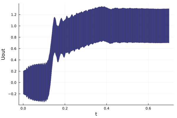
Since we are only interested in the behavior of $U_{out}$, we could use an algorithm based on the support function (see, e.g., Girard and Le Guernic [GL08], which can be used as LGG09 in this library), or the decomposition-based algorithm BFFPSV18 with the options alg=BFFPSV18(δ=1e-3, dim=statedim(P), vars=[η])). These options will use an interval (1D) decomposition of the state space and only compute the flowpipe associated with variable $η$.