Vehicle Platoon

Overview

System type: Linear hybrid system
State dimension: 9 + time
Application domain: Autonomous driving

Model description

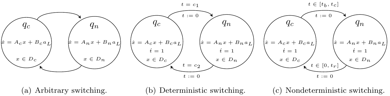
This benchmark considers a platoon of three vehicles following each other. In addition, loss of communication between the vehicles can occur. The hybrid model shown below has two operational modes, connected ($q_c$) and disconnected (or not connected, $q_n$).

There are three scenarios for the loss of communication:

PLAA01 (arbitrary loss) (left model): The loss of communication can occur at any time. This includes the possibility of no communication at all.

PLADxy (loss at deterministic times) (central model): The loss of communication occurs at deterministic points in time, which are determined by clock constraints $c_1$ and $c_2$. The clock $t$ is reset when communication is lost and when it is reestablished. Note that here the transitions have must-semantics, i.e., they take place as soon as possible. We will consider PLAD01: $c_1 = c_2 = 5$.

PLANxy (loss at nondeterministic times): The loss of communication occurs during time intervals $t ∈ [t_b, t_c]$. The clock $t$ is reset when communication is lost and when it is reestablished. Communication is reestablished at any time $t ∈ [0, t_r]$. This scenario covers loss of communication after an arbitrarily long time $t ≥ t_c$ by reestablishing communication in zero time. We will consider PLAN01: $t_b = 10$, $t_c = 20$, and $t_r = 20$.

using ReachabilityAnalysis, SparseArrays, Symbolics

const var = @variables x[1:9] t;

In this notebook we only consider the case of deterministic switching (central model). Next we develop this model. It is convenient to create two independent functions, platoon_connected and platoon_disconnected, which describe the dynamics of the connected (resp. disconnected) modes.

Dynamics of the "connected" platoon

function platoon_connected(; deterministic_switching::Bool=true, c1=5.0)
    n = 9 + 1

    # x' = Ax + Bu + c
    A = Matrix{Float64}(undef, n, n)
    A[1, :] = [0, 1.0, 0, 0, 0, 0, 0, 0, 0, 0]
    A[2, :] = [0, 0, -1.0, 0, 0, 0, 0, 0, 0, 0]
    A[3, :] = [1.6050, 4.8680, -3.5754, -0.8198, 0.4270, -0.0450, -0.1942, 0.3626, -0.0946, 0.0]
    A[4, :] = [0, 0, 0, 0, 1.0, 0, 0, 0, 0, 0]
    A[5, :] = [0, 0, 1.0, 0, 0, -1.0, 0, 0, 0, 0]
    A[6, :] = [0.8718, 3.8140, -0.0754, 1.1936, 3.6258, -3.2396, -0.5950, 0.1294, -0.0796, 0.0]
    A[7, :] = [0, 0, 0, 0, 0, 0, 0, 1.0, 0, 0]
    A[8, :] = [0, 0, 0, 0, 0, 1.0, 0, 0, -1.0, 0]
    A[9, :] = [0.7132, 3.5730, -0.0964, 0.8472, 3.2568, -0.0876, 1.2726, 3.0720, -3.1356, 0.0]
    A[10, :] = [0, 0, 0, 0, 0, 0, 0, 0, 0, 0.0] # t' = 1

    if deterministic_switching
        invariant = HalfSpace(t <= c1, var)
    else
        invariant = Universe(n)
    end

    # acceleration of the lead vehicle + time
    B = sparse([2], [1], [1.0], n, 1)
    U = Hyperrectangle(; low=[-9.0], high=[1.0])
    c = [0, 0, 0, 0, 0, 0, 0, 0, 0, 1.0]
    @system(x' = A * x + B * u + c, x ∈ invariant, u ∈ U)
end;

Dynamics of the "disconnected" platoon

function platoon_disconnected(; deterministic_switching::Bool=true, c2=5.0)
    n = 9 + 1

    # x' = Ax + Bu + c
    A = Matrix{Float64}(undef, n, n)
    A[1, :] = [0, 1.0, 0, 0, 0, 0, 0, 0, 0, 0]
    A[2, :] = [0, 0, -1.0, 0, 0, 0, 0, 0, 0, 0]
    A[3, :] = [1.6050, 4.8680, -3.5754, 0, 0, 0, 0, 0, 0, 0]
    A[4, :] = [0, 0, 0, 0, 1.0, 0, 0, 0, 0, 0]
    A[5, :] = [0, 0, 1.0, 0, 0, -1.0, 0, 0, 0, 0]
    A[6, :] = [0, 0, 0, 1.1936, 3.6258, -3.2396, 0, 0, 0, 0.0]
    A[7, :] = [0, 0, 0, 0, 0, 0, 0, 1.0, 0, 0]
    A[8, :] = [0, 0, 0, 0, 0, 1.0, 0, 0, -1.0, 0]
    A[9, :] = [0.7132, 3.5730, -0.0964, 0.8472, 3.2568, -0.0876, 1.2726, 3.0720, -3.1356, 0.0]
    A[10, :] = [0, 0, 0, 0, 0, 0, 0, 0, 0, 0.0] # t' = 1

    if deterministic_switching
        invariant = HalfSpace(t <= c2, var)
    else
        invariant = Universe(n)
    end

    # acceleration of the lead vehicle + time
    B = sparse([2], [1], [1.0], n, 1)
    U = Hyperrectangle(; low=[-9.0], high=[1.0])
    c = [0, 0, 0, 0, 0, 0, 0, 0, 0, 1.0]
    @system(x' = A * x + B * u + c, x ∈ invariant, u ∈ U)
end;

Hybrid system

function platoon(; deterministic_switching::Bool=true,
                 c1=5.0,  # clock constraint
                 c2=5.0,  # clock constraint
                 tb=10.0,  # lower bound for loss of communication
                 tc=20.0,  # upper bound for loss of communication
                 tr=20.0)  # reset time

    # three variables for each vehicle, (ei, d(et)/dt, ai) for
    # (spacing error, relative velocity, speed), and the last dimension is time
    n = 9 + 1

    # transition graph
    automaton = GraphAutomaton(2)
    add_transition!(automaton, 1, 2, 1)
    add_transition!(automaton, 2, 1, 2)

    # modes
    mode1 = platoon_connected(; deterministic_switching=deterministic_switching, c1=c1)
    mode2 = platoon_disconnected(; deterministic_switching=deterministic_switching, c2=c2)
    modes = [mode1, mode2]

    # common reset
    reset = Dict(n => 0.0)

    # transition l1 -> l2
    if deterministic_switching
        guard = Hyperplane(t == c1, var)
    else
        guard = HPolyhedron([tb <= t, t <= tc], var)
    end
    t1 = ConstrainedResetMap(n, guard, reset)

    # transition l2 -> l1
    if deterministic_switching
        guard = Hyperplane(t == c2, var)
    else
        guard = HalfSpace(t <= tr, var)
    end
    t2 = ConstrainedResetMap(n, guard, reset)

    resetmaps = [t1, t2]
    H = HybridSystem(automaton, modes, resetmaps, [AutonomousSwitching()])

    # initial condition: at the origin in mode 1
    X0 = BallInf(zeros(n), 0.0)
    initial_condition = [(1, X0)]

    return IVP(H, initial_condition)
end;

Specification

The goal is to prove that the minimum distance between vehicles is preserved. The choice of the coordinate system is such that the minimum distance is a negative value. We consider the following family of specifications:

BNDxy: Bounded time (no explicit bound on the number of transitions): For all $t ∈ [0, 20] [s]$,

$x_1(t) ≥ −d_{min} [m]$
$x_4(t) ≥ −d_{min} [m]$
$x_7(t) ≥ −d_{min} [m]$

Concretely, we choose the following two cases of increasing difficulty:

BND42: $d_{min} = 42$.

BND30: $d_{min} = 30$.

function dmin_specification(sol, dmin)
    return (-ρ(sparsevec([1], [-1.0], 10), sol) ≥ -dmin) &&
           (-ρ(sparsevec([4], [-1.0], 10), sol) ≥ -dmin) &&
           (-ρ(sparsevec([7], [-1.0], 10), sol) ≥ -dmin)
end

prob_PLAD01 = platoon();

Results

PLAD01 - BND42

This scenario can be solved using a hyperrectangular set representation with step size $δ = 0.01$. We use a template that contains all box (i.e., canonical) directions in the ambient space of the state space (plus time), $\mathbb{R}^{10}$. There are $20$ such directions, two for each coordinate:

boxdirs = BoxDirections(10)
length(boxdirs)

alg = BOX(; δ=0.01)
sol_PLAD01_BND42 = solve(prob_PLAD01;
                         alg=alg,
                         clustering_method=BoxClustering(1),
                         intersection_method=TemplateHullIntersection(boxdirs),
                         intersect_source_invariant=false,
                         T=20.0);

We verify that the specification holds:

@assert dmin_specification(sol_PLAD01_BND42, 42) "the property should be proven"

In more detail, we can check how far the flowpipe is from violating the property. The specification requires that each of the following quantities is greater than -dmin = -42.

Minimum of $x_1(t)$:

-ρ(sparsevec([1], [-1.0], 10), sol_PLAD01_BND42)

-41.366377912095516

Minimum of $x_4(t)$:

-ρ(sparsevec([4], [-1.0], 10), sol_PLAD01_BND42)

-35.52209043200976

Minimum of $x_7(t)$:

-ρ(sparsevec([7], [-1.0], 10), sol_PLAD01_BND42)

-21.601435520428574

Next, we plot variable $x_1$ over time.

using Plots, LaTeXStrings

fig = plot(sol_PLAD01_BND42; vars=(0, 1), xlab=L"t", ylab=L"x_1", title="PLAD01 - BND42", lw=0.1)
plot!(x -> x, x -> -42.0, 0.0, 20.0; linewidth=2, color="red", ls=:dash, leg=nothing)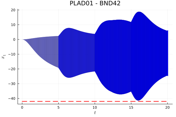

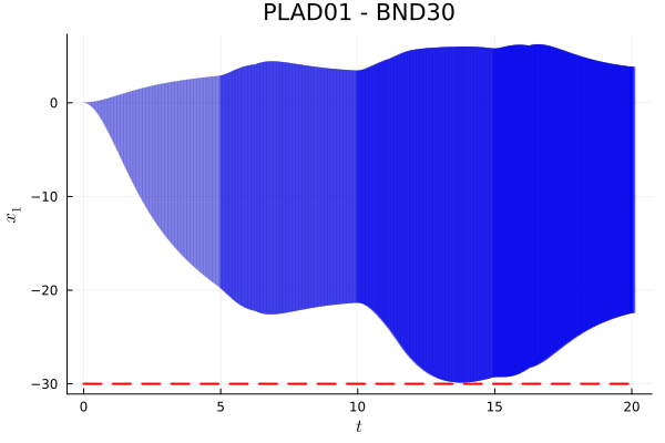
PLAD01 - BND30

Note that the previous solution obtained for PLAD01 - BND42 does not verify the BND30 specifications since, for example, the minimum of variable $x_4(t)$ is $≈ -35.52$, which is below the given bound $-d_{min} = -30$. As a consequence, to prove the safety properties for this scenario, we have to use a solver with more precision. Instead of the BOX algorithm, we will use LGG09 with step-size $δ = 0.03$ and octagonal template directions. There are 200 such directions:

octdirs = OctDirections(10)
length(octdirs)

Performance tip

The increase in the number of directions implies an increase in run time. Since evaluating the 200 directions of the template is quite expensive, we use a concrete set after the discretization (instead of using a lazy discretization). This is achieved by passing the option approx_model=Forward(setops=octdirs) to the LGG09 algorithm, specifying that we want to oveapproximate the initial set of the set-based recurrence with an octagonal template. In this example, this option gives a gain in runtime of $~30\%$, without a noticeable loss in precision.

alg = LGG09(; δ=0.03, template=octdirs, approx_model=Forward(; setops=octdirs))
sol_PLAD01_BND30 = solve(prob_PLAD01;
                         alg=alg,
                         clustering_method=LazyClustering(1),
                         intersection_method=TemplateHullIntersection(octdirs),
                         intersect_source_invariant=false,
                         T=20.0);

We verify that the specification holds:

@assert dmin_specification(sol_PLAD01_BND30, 30) "the property should be proven"

Check in more detail how close the flowpipe is to the safety conditions:

Minimum of $x_1(t)$:

-ρ(sparsevec([1], [-1.0], 10), sol_PLAD01_BND30)

-29.862721575258067

Minimum of $x_4(t)$:

-ρ(sparsevec([4], [-1.0], 10), sol_PLAD01_BND30)

-26.167902001889445

Minimum of $x_7(t)$:

-ρ(sparsevec([7], [-1.0], 10), sol_PLAD01_BND30)

-12.696657569596857

Finally, we plot variable $x_1$ over time again.

fig = plot(sol_PLAD01_BND30; vars=(0, 1), xlab=L"t", ylab=L"x_1", title="PLAD01 - BND30", lw=0.1)
plot!(x -> x, x -> -30.0, 0.0, 20.0; linewidth=2, color="red", ls=:dash, leg=nothing)