Electromechanical brake

Model description

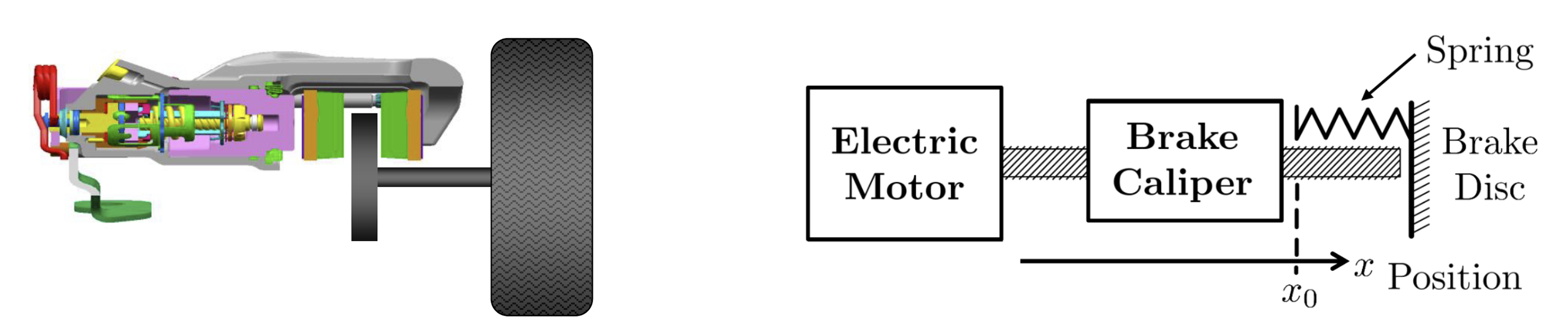
This system models an electromechanical brake, which works as in the following image.

The system is described by linear differential equations:

\[\begin{aligned} \dot{x}(t) &= Ax(t) + Bu(t),\qquad u(t) ∈ \mathcal{U} \\ y(t) &= Cx(t) \end{aligned}\]

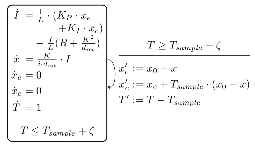
A hybrid-automaton model is depicted below.

There are two versions of this benchmark:

• Time-varying inputs: The inputs can change arbitrarily over time: $\forall t: u(t) ∈ \mathcal{U}$.

• Constant inputs: The inputs are only uncertain in the initial value, and constant over time: $u(0) ∈ \mathcal{U}$, $\dot{u}(t) = 0.$

using ReachabilityAnalysis, SparseArrays

Common functionality between model variants

The following code is shared between all model variants.

function embrake_common(; A, Tsample, ζ, x0)
    # continuous system
    EMbrake = @system(x' = A * x)

    # initial condition
    X₀ = Singleton([0.0, 0, 0, 0])

    # reset map
    Ar = sparse([1, 2, 3, 4, 4], [1, 2, 2, 2, 4], [1.0, 1.0, -1.0, -Tsample, 1.0], 4, 4)
    br = sparsevec([3, 4], [x0, Tsample * x0], 4)
    reset_map(X) = Ar * X + br

    # hybrid system with clocked affine dynamics
    ha = HACLD1(EMbrake, reset_map, Tsample, ζ)
    return IVP(ha, X₀)
end;

Fixed parameters

The model without parameter variation is defined below.

function embrake_no_pv(; Tsample=1.E-4, ζ=1e-6, x0=0.05)
    # model's constants
    L = 1.e-3
    KP = 10000.0
    KI = 1000.0
    R = 0.5
    K = 0.02
    drot = 0.1
    i = 113.1167

    # state variables: [I, x, xe, xc]
    A = Matrix([-(R + K^2 / drot)/L 0 KP/L KI/L;
                K / i/drot 0 0 0;
                0 0 0 0;
                0 0 0 0])

    return embrake_common(; A=A, Tsample=Tsample, ζ=ζ, x0=x0)
end;

Parameter variation

The model with parameter variation described below consists of changing only one coefficient, which corresponds to the Flow* settings in ^[SO15].

function embrake_pv_1(; Tsample=1.E-4, ζ=1e-6, Δ=3.0, x0=0.05)
    # model's constants
    L = 1.e-3
    KP = 10000.0
    KI = 1000.0
    R = 0.5
    K = 0.02
    drot = 0.1
    i = 113.1167
    p = 504.0 + (-Δ .. Δ)

    # state variables: [I, x, xe, xc]
    A = IntervalMatrix([-p 0 KP/L KI/L;
                        K / i/drot 0 0 0;
                        0 0 0 0;
                        0 0 0 0])

    return embrake_common(; A=A, Tsample=Tsample, ζ=ζ, x0=x0)
end;

Extended parameter variation

In the following model, considered in ^[SO15], we vary all constants by χ% with respect to their nominal values. The variation percentage defaults to 5%.

function embrake_pv_2(; Tsample=1.E-4, ζ=1e-6, x0=0.05, χ=5.0)
    # model's constants
    Δ = -χ / 100 .. χ / 100
    L = 1.e-3 * (1 + Δ)
    KP = 10000.0 * (1 + Δ)
    KI = 1000.0 * (1 + Δ)
    R = 0.5 * (1 + Δ)
    K = 0.02 * (1 + Δ)
    drot = 0.1 * (1 + Δ)
    i = 113.1167 * (1 + Δ)

    # state variables: [I, x, xe, xc]
    A = IntervalMatrix([-(R + K^2 / drot)/L 0 KP/L KI/L;
                        K / i/drot 0 0 0;
                        0 0 0 0;
                        0 0 0 0])

    return embrake_common(; A=A, Tsample=Tsample, ζ=ζ, x0=x0)
end;

References