Production/Destruction

Model description

A production-destruction system consists of an ordinary differential equation and two constraints: positivity and conservativity. It means that the system states are quantities which are always positive and their sum is constant. This particular family of systems is often used to test the stability of integration schemes.

As proposed by Michaelis-Menten theory ^[KM18], a model for three quantities can be defined as follows:

\[\begin{aligned} \dot{x} &= \dfrac{-xy}{1+x} \\[2mm] \dot{y} &= \dfrac{xy}{1+x} - a y \\[2mm] \dot{z} &= a y \end{aligned}\]

with nominal value $a = 0.3$ and an initial condition $x(0) = 9.98$, $y(0) = 0.01$, and $z(0) = 0.01$. In this model, $x$ represents the nutrients, $y$ the phytoplankton, and $z$ the detritus. In this case study, we analyze the behavior of the system subject to uncertainties in the initial condition and/or the model's parameter $a$.

Specification

The solution should satisfy the following two constraints:

• Positivity: $x(t)$, $y(t)$, $z(t)$ are positive, and
• Conservativity: $x(t) + y(t) + z(t) = 10$ for all $t ≥ 0$.

Here we are interested in computing the reachable tube until the time horizon $T=100$ and to verify the constraints $10 ∈ x+y+z$ and $x, y, z ≥ 0$ at $T = 100$. Three setups are considered, depending on the source of bounded uncertainties:

• Case I: $x(0) ∈ [9.5, 10.0]$, i.e., uncertainty in the initial condition;
• Case P: $a ∈ [0.296, 0.304]$, i.e., uncertainty in the parameter value;
• Case I & P: $x(0) ∈ [9.5, 10.0]$ and $a ∈ [0.296, 0.304]$, i.e., both uncertainties are present.

The reachability settings considered above are a variation of those in ^{[ARCHCOMP20_NLN]}. Note that variables $x$ and $y$ converge towards zero, so the final volume can be used as a quality measure of the overapproximation.

We consider two measures of quality of the approximation: the volume of the box ($x × y × z$) enclosing the final states (at $T = 100$) and the total time of computation for evolution and verification. These results are obtained for the three setups.

We discuss the implementation of each constraint satisfaction problem, beginning by defining the positive orthant in three-dimensional space, positive_orthant, as an unbounded polyhedron in constraint representation.

using ReachabilityAnalysis, Symbolics

@variables x y z
positive_orthant = HPolyhedron([x >= 0, y >= 0, z >= 0], [x, y, z]);

Given a set $X ⊆ \mathbb{R}^n$, checking whether the positivity constraint holds corresponds to checking whether $X$ is included in the positive orthant. This computation can be done efficiently using the support function, which is available in LazySets.jl. Multiple dispatch takes care based on the types of the arguments in the call X ⊆ positive_orthant depending on the type of $X$.

On the other hand, given a set $X$, a quick way to check the conservativity constraint is to first overapproximate $X$ with a box, then represent this box as a product-of-intervals (IntervalBox) B, and finally take the Minkowski sum of each interval, using sum(B). This check is only sufficient; splitting $X$ can be used to refine the check.

The verification problem is summarized in the function prod_dest_verif. It receives the solution of a reachability problem represented with a Taylor-model flowpipe and two optional arguments that specify the time horizon T, which defaults to 100, and the conservativity condition given a target value target, which defaults to 10. The function returns the tuple (sat, vol). The first output, sat, is true if and only if the positivity and conservativity conditions are satisfied at the time horizon T. The second output, vol, corresponds to the volume of the box overapproximation of the final reach set.

function prod_dest_verif(sol; T=100.0, target=10.0)
    # obtain the final reach set and project onto the state variables x, y, z
    Xh = box_approximation(sol(T))
    X = project(Xh; vars=(1, 2, 3))

    # check that all variables are nonnegative
    nonnegative = X ⊆ positive_orthant

    # compute the volume
    vol = volume(X)

    # check that the target belongs to the Minkowski sum of the projections
    # onto each coordinate
    B = convert(IntervalBox, X) # get a product-of-intervals representation
    contains_target = target ∈ sum(B)

    return nonnegative && contains_target, vol
end;

Analysis & Results

Case I

Case I corresponds to uncertainty in the initial states. We begin by writing the system of differential equations in the function prod_dest_I!.

@taylorize function prod_dest_I!(du, u, p, t)
    local a = 0.3
    x, y, z = u

    xyx = (x * y) / (1 + x)
    ay = a * y

    du[1] = -xyx
    du[2] = xyx - ay
    du[3] = ay
    return du
end

The initial states are uncertain in dimension $x$.

X0 = Hyperrectangle(; low=[9.5, 0.01, 0.01], high=[10, 0.01, 0.01])
prob = @ivp(x' = prod_dest_I!(x), dim:3, x(0) ∈ X0);

Analysis

sol = solve(prob; T=100.0, alg=TMJets(; abstol=1e-12, orderT=6, orderQ=1));

Verify that the specification holds:

property, vol = prod_dest_verif(sol)
@assert property "the property should be proven"
vol

1.3472995827239226e-16

Results

We plot $z$ over time.

using Plots

fig = plot(sol; vars=(0, 3), lc=:orange, c=:orange, alpha=0.3, lab="I", xlab="t", ylab="z")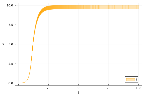

Case P

For the case of an uncertain parameter, we add a new state variable that corresponds to $a$, with constant (zero) dynamics.

@taylorize function prod_dest_IP!(du, u, p, t)
    x, y, z, a = u[1], u[2], u[3], u[4]

    xyx = (x * y) / (1 + x)
    ay = a * y

    du[1] = -xyx
    du[2] = xyx - ay
    du[3] = ay
    du[4] = zero(a)
    return du
end

X0 = Hyperrectangle(; low=[9.98, 0.01, 0.01, 0.296], high=[9.98, 0.01, 0.01, 0.304])
prob = @ivp(x' = prod_dest_IP!(x), dim:4, x(0) ∈ X0);

Analysis

sol = solve(prob; T=100.0, alg=TMJets(; abstol=9e-13, orderT=6, orderQ=1));

Verify that the specification holds:

property, vol = prod_dest_verif(sol)
@assert property "the property should be proven"
vol

1.4702608588936523e-24

Results

We plot $z$ over time.

fig = plot(sol; vars=(0, 3), lc=:blue, c=:blue, alpha=0.3, lab="P", xlab="t", ylab="z")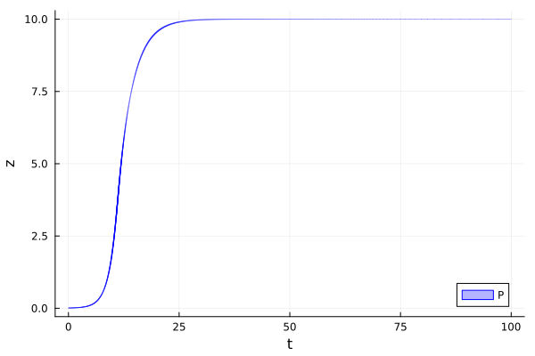

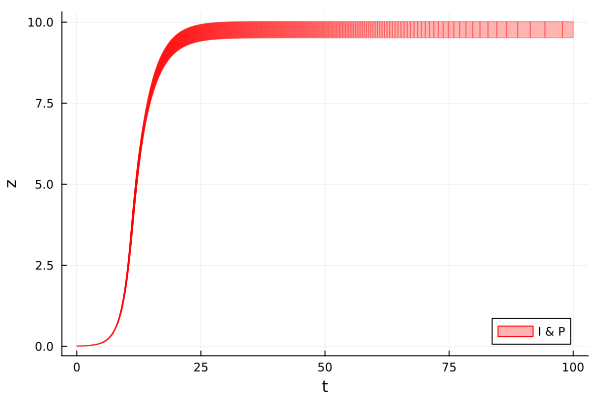
Case I & P

When uncertainty in both the initial states and the parameters are present, we can reuse the function prod_dest_IP!, but setting an uncertain initial condition and an uncertain parameter. Recall that we are interested in $x(0) ∈ [9.5, 10.0]$ and $a ∈ [0.296, 0.304]$.

X0 = Hyperrectangle(; low=[9.5, 0.01, 0.01, 0.296], high=[10, 0.01, 0.01, 0.304])
prob = @ivp(x' = prod_dest_IP!(x), dim:4, x(0) ∈ X0);

Analysis

sol = solve(prob; T=100.0, alg=TMJets(; abstol=1e-12, orderT=6, orderQ=1));

Verify that the specification holds:

property, vol = prod_dest_verif(sol)
@assert property "the property should be proven"
vol

2.703239675065678e-16

Results

We plot $z$ over time.

fig = plot(sol; vars=(0, 3), lc=:red, c=:red, alpha=0.3, lab="I & P", xlab="t", ylab="z")

References