Spacecraft

Model description

Spacecraft rendezvous is a perfect use case for formal verification of hybrid systems with nonlinear dynamics since mission failure can cost lives and is extremely expensive. This benchmark is taken from ^[CM17] but adapted to the settings of ARCH-COMP ^[ARCHCOMP].

The nonlinear differential equations describe the two-dimensional, planar motion of the space-craft on an orbital plane towards a space station:

\[\begin{aligned} \dot{x} &= v_x \\ \dot{y} &= v_y \\ \dot{v_x} &= n^2x + 2nv_y + \dfrac{μ}{r^2} - \dfrac{μ}{r_c^3} (r +x) + \dfrac{u_x}{m_c} \\ \dot{v_y} &= n^2y - 2nv_x - \dfrac{μ}{r_c^3}y + \dfrac{u_y}{m_c} \end{aligned}\]

The model consists of a 2D position (relative to the target) $x$, $y$ [m], time $t$ [min], as well as horizontal and vertical velocity $v_x$, $v_y$ [m / min]. The parameters are $µ = 3.986 × 10^{14} × 60^2$ [m$^3$ / min$^2$], $r = 42164 × 10^3$ [m], $m_c = 500$ [kg], $n = \sqrt{\dfrac{μ}{r^3}}$ and $r_c = \sqrt{(r + x)^2 + y^2}$.

The hybrid nature of this benchmark originates from a switched controller. In particular, the modes are approaching ($x ∈ [−1000, −100]$ [m]), rendezvous attempt ($x ≥ −100$ [m]), and aborting. A transition to mode aborting occurs nondeterministically at $t ∈ [120, 150]$ [min].

The linear feedback controllers for the different modes are defined as $\binom{u_x}{u_y} = K_1 s$ for mode approaching, and $\binom{u_x}{u_y} = K_2 s$ for mode rendezvous attempt, where $s = (x, y, v_x, v_y)^T$ is the vector of system states. In the mode aborting, the system is uncontrolled: $\binom{u_x}{u_y} = \binom{0}{0}$. The feedback matrices $K_i$ were determined with an LQR-approach applied to the linearized system dynamics, which resulted in the following numerical values:

\[\begin{aligned} K_1 &= \begin{pmatrix} −28.8287 & 0.1005 & −1449.9754 & 0.0046 \\ −0.087 & −33.2562 & 0.00462 & −1451.5013 \end{pmatrix} \\ K_2 &= \begin{pmatrix} −288.0288 & 0.1312 & −9614.9898 & 0 \\ −0.1312 & −288 & 0 & −9614.9883 \end{pmatrix} \end{aligned}\]

using ReachabilityAnalysis  # !jl

const μ = 3.986e14 * 60^2
const r = 42164.0e3
const r² = r^2
const mc = 500.0
const n² = μ / r^3
const n = sqrt(n²)

const two_n = 2 * n
const μ_r² = μ / r²

const K₁ = [-28.8287 0.1005 -1449.9754 0.0046 0.0;
            -0.087 -33.2562 0.00462 -1451.5013 0.0]
const K₂ = [-288.0288 0.1312 -9614.9898 0.0 0.0;
            -0.1312 -288.0 0.0 -9614.9883 0.0]

const K₁mc = K₁ / mc
const K₂mc = K₂ / mc

function mymul!(v, A, x)  # helper function for matrix-vector multiplication
    @inbounds for ind in eachindex(v)
        v[ind] = zero(x[1])
        for jind in eachindex(x)
            v[ind] += A[ind, jind] * x[jind]
        end
    end
    return nothing
end;

Dynamics in the approaching mode

@taylorize function spacecraft_approaching!(du, u, p, time)
    x, y, vx, vy, t = u

    rx = r + x
    rx² = rx^2
    y² = y^2
    rc = sqrt(rx² + y²)
    rc³ = rc^3
    μ_rc³ = μ / rc³

    uxy = Vector{typeof(x)}(undef, 2)
    mymul!(uxy, K₁mc, u)

    # x' = vx
    du[1] = vx

    # y' = vy
    du[2] = vy

    # vx' = n²x + 2n*vy + μ/(r^2) - μ/(rc^3)*(r+x) + ux/mc
    du[3] = (n² * x + two_n * vy) + ((μ_r² - μ_rc³ * rx) + uxy[1])

    # vy' = n²y - 2n*vx - μ/(rc^3)y + uy/mc
    du[4] = (n² * y - two_n * vx) - (μ_rc³ * y - uxy[2])

    # t' = 1
    du[5] = one(t)

    return du
end

Dynamics in the rendezvous attempt mode

@taylorize function spacecraft_attempt!(du, u, p, time)
    x, y, vx, vy, t = u

    rx = r + x
    rx² = rx^2
    y² = y^2
    rc = sqrt(rx² + y²)
    rc³ = rc^3
    μ_rc³ = μ / rc³

    uxy = Vector{typeof(x)}(undef, 2)
    mymul!(uxy, K₂mc, u)

    # x' = vx
    du[1] = vx

    # y' = vy
    du[2] = vy

    # vx' = n²x + 2n*vy + μ/(r^2) - μ/(rc^3)*(r+x) + ux/mc
    du[3] = (n² * x + two_n * vy) + ((μ_r² - μ_rc³ * rx) + uxy[1])

    # vy' = n²y - 2n*vx - μ/(rc^3)y + uy/mc
    du[4] = (n² * y - two_n * vx) - (μ_rc³ * y - uxy[2])

    # t' = 1
    du[5] = one(t)

    return du
end

Dynamics in the aborting mode

@taylorize function spacecraft_aborting!(du, u, p, time)
    x, y, vx, vy, t = u

    rx = r + x
    rx² = rx^2
    y² = y^2
    rc = sqrt(rx² + y²)
    rc³ = rc^3
    μ_rc³ = μ / rc³

    # x' = vx
    du[1] = vx

    # y' = vy
    du[2] = vy

    # vx' = n²x + 2n*vy + μ/(r^2) - μ/(rc^3)*(r+x)
    du[3] = (n² * x + two_n * vy) + (μ_r² - μ_rc³ * rx)

    # vy' = n²y - 2n*vx - μ/(rc^3)y
    du[4] = (n² * y - two_n * vx) - μ_rc³ * y

    # t' = 1
    du[5] = one(t)

    return du
end

Hybrid system

To model the system as a hybrid automaton, it is useful to work with symbolic state variables.

using Symbolics

const var = @variables x y vx vy t

function spacecraft(; abort_time=(120.0, 150.0))
    n = 4 + 1  # number of variables
    t_abort_lower, t_abort_upper = abort_time

    automaton = GraphAutomaton(3)

    # mode 1 (approaching)
    invariant = HalfSpace(x <= -100, var)
    approaching = @system(x' = spacecraft_approaching!(x), dim:5, x ∈ invariant)

    # mode 2 (rendezvous attempt)
    invariant = HalfSpace(x >= -100, var)
    attempt = @system(x' = spacecraft_attempt!(x), dim:5, x ∈ invariant)

    # mode 3 (aborting)
    invariant = Universe(n)
    aborting = @system(x' = spacecraft_aborting!(x), dim:5, x ∈ invariant)

    # transition "approach" -> "rendezvous attempt"
    add_transition!(automaton, 1, 2, 1)
    guard = HalfSpace(x >= -100, var)
    t1 = @map(x -> x, dim:n, x ∈ guard)

    # transition "approach" -> "abort"
    add_transition!(automaton, 1, 3, 2)
    guard_time = HPolyhedron([t >= t_abort_lower, t <= t_abort_upper], var)
    t2 = @map(x -> x, dim:n, x ∈ guard_time)

    # transition "rendezvous attempt" -> "abort"
    add_transition!(automaton, 2, 3, 3)
    t3 = @map(x -> x, dim:n, x ∈ guard_time)

    H = HybridSystem(; automaton=automaton,
                     modes=[approaching, attempt, aborting],
                     resetmaps=[t1, t2, t3])

    # initial condition in mode 1
    X0 = Hyperrectangle([-900.0, -400, 0, 0, 0], [25.0, 25, 0, 0, 0])
    init = [(1, X0)]

    return InitialValueProblem(H, init)
end;

Specification

The spacecraft starts from the initial set $x ∈ [−925, −875]$ [m], $y ∈ [−425, −375]$ [m], $vx = 0$ [m/min], and $vy = 0$ [m/min]. For the considered time horizon of $t ∈ [0, 200]$ [min], the following specifications have to be satisfied:

• Line-of-sight: In mode rendezvous attempt, the spacecraft has to stay inside the line-of-sight cone $L = \{\binom{x}{y} | (x ≥ −100) ∧ (y ≥ x \tan(30°)) ∧ (−y ≥ x \tan(30°))\}$.

• Collision avoidance: In mode aborting, the spacecraft has to avoid a collision with the target, which is modeled as a box $B$ with $0.2$ [m] edge length and the center placed at the origin.

• Velocity constraint: In mode rendezvous attempt, the absolute velocity has to stay below $3.3$ [m/min]: $\sqrt{v^2_x + v^2_y} ≤ 3.3$ [m/min].

const tan30 = tand(30)

LineOfSightCone = HPolyhedron([x >= -100, y >= x * tan30, -y >= x * tan30], var)

target = BallInf(zeros(2), 0.2)

function line_of_sight(sol)
    all_idx = findall(x -> x == 2, location.(sol))  # "rendezvous attempt" mode
    for idx in all_idx
        if !all(set(R) ⊆ LineOfSightCone for R in sol[idx][2:end])
            return false
        end
    end
    return true
end

function collision_avoidance(sol)
    all_idx = findall(x -> x == 3, location.(sol))  # "aborting" mode
    for idx in all_idx
        if !all(isdisjoint(set(Projection(R, [1, 2])), target) for R in sol[idx])
            (set(Projection(R, [1, 2])) for R in sol[idx])
            return false
        end
    end
    return true
end

function absolute_velocity(R)
    vx, vy = 3, 4
    vx2 = set(overapproximate(project(R; vars=(vx,)), Interval))
    vy2 = set(overapproximate(project(R; vars=(vy,)), Interval))
    return sqrt(vx2.dat + vy2.dat)
end

function velocity_constraint(sol)
    all_idx = findall(x -> x == 2, location.(sol))  # "rendezvous attempt" mode
    for idx in all_idx
        # maximum velocity measured in m/min
        if !all(absolute_velocity(R) < 0.055 * 60.0 for R in sol[idx])
            return false
        end
    end
    return true
end;

Analysis

The transition to the aborting mode is handled by clustering the flowpipe into 25 boxes.

function solve_spacecraft(prob; k=25, s=missing)
    # transition from mode 1 to mode 2
    sol12 = solve(prob;
                  tspan=(0.0, 200.0),
                  alg=TMJets21a(; abstol=1e-5, maxsteps=10_000, orderT=5, orderQ=1,
                                disjointness=BoxEnclosure()),
                  max_jumps=1,
                  intersect_source_invariant=false,
                  intersection_method=TemplateHullIntersection(BoxDirections(5)),
                  clustering_method=LazyClustering(1),
                  disjointness_method=BoxEnclosure())
    sol12jump = overapproximate(sol12[2](120 .. 150), Zonotope)
    t0 = tstart(sol12jump[1])
    sol12jump_c = cluster(sol12jump, 1:length(sol12jump), BoxClustering(k, s))

    # transition from mode 2 to mode 3
    H = system(prob)
    sol3 = solve(IVP(mode(H, 3), [set(X) for X in sol12jump_c]);
                 tspan=(t0, 200.0),
                 alg=TMJets21a(; abstol=1e-10, orderT=7, orderQ=1, disjointness=BoxEnclosure()))
    d = Dict{Symbol,Any}(:loc_id => 3)
    F12 = [fp for fp in sol12.F]
    F23 = [Flowpipe(fp.Xk, d) for fp in sol3.F]
    return HybridFlowpipe(vcat(F12, F23))
end

prob = spacecraft()
sol = solve_spacecraft(prob; k=25, s=missing)
solz = overapproximate(sol, Zonotope);

┌ Warning: maximum number of jumps reached; try increasing `max_jumps`
└ @ ReachabilityAnalysis ~/work/ReachabilityAnalysis.jl/ReachabilityAnalysis.jl/src/Hybrid/solve.jl:143

Now we verify the specification. Verifying the collision avoidance requires more effort, so here we do not manage to prove this property.

@assert line_of_sight(solz) "the property should be proven"
@assert !collision_avoidance(solz) "the property cannot be proven with these settings"
@assert velocity_constraint(solz) "the property should be proven"

Results

using Plots, Plots.PlotMeasures, LaTeXStrings

fig = plot(solz; vars=(1, 2), xlab="x", ylab="y")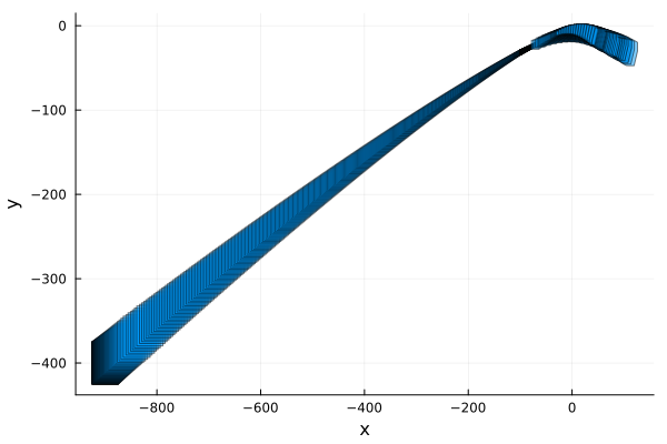

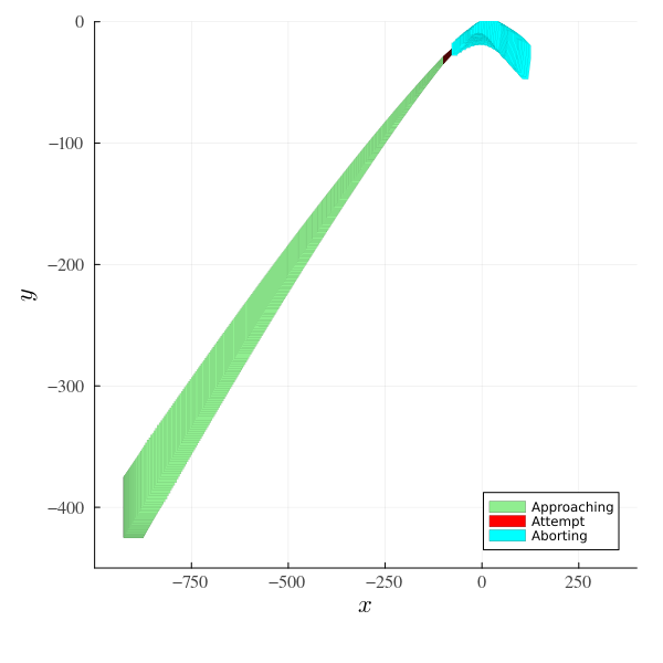
Note that in the previous plot, it is not specified which reach set corresponds to which mode. After finding the location (mode of the hybrid system) associated to each reach set of the solution, we can plot each one using different colors. The plotting code is more sophisticated than before, and is an example of finer control of the options used to plot the flowpipes.

idx_approaching = findall(x -> x == 1, location.(solz))
idx_attempt = findall(x -> x == 2, location.(solz))
idx_aborting = findall(x -> x == 3, location.(solz))

fig = plot(; legend=:bottomright, tickfont=font(10, "Times"), guidefontsize=15,
           xlab=L"x", ylab=L"y", lw=0.0, xtick=[-750, -500, -250, 0, 250.0],
           ytick=[-400, -300, -200, -100, 0.0], xlims=(-1000.0, 400.0), ylims=(-450.0, 0.0),
           size=(600, 600), bottom_margin=6mm, left_margin=2mm, right_margin=4mm, top_margin=3mm)

plot!(fig, solz[idx_approaching[1]]; vars=(1, 2), lw=0.0, color=:lightgreen, alpha=1,
      lab="Approaching")
for k in idx_approaching[2:end]
    plot!(fig, solz[k]; vars=(1, 2), lw=0.0, color=:lightgreen, alpha=1)
end

plot!(fig, solz[idx_attempt[1]]; vars=(1, 2), lw=0.0, color=:red, alpha=1, lab="Attempt")
for k in idx_attempt[2:end]
    plot!(fig, solz[k]; vars=(1, 2), lw=0.0, color=:red, alpha=1)
end

plot!(fig, solz[idx_aborting[1]]; vars=(1, 2), lw=0.0, color=:cyan, alpha=1, lab="Aborting")
for k in idx_aborting[2:end]
    plot!(fig, solz[k]; vars=(1, 2), lw=0.0, color=:cyan, alpha=1)
end

fig

References