Set propagation in discrete time
Our motivating example is to solve the following simple linear set-based recurrence
\[X_{k+1} = M(θ) X_k, \qquad 0 ≤ k ≤ 50, X_0 = [0.8, 1.2] \times [0.8, 1.2] ⊆ \mathbb{R}^2\]
Let $θ ∈ [0, 2 π]$ be an equally spaced vector of length $50$, and $M(θ)$ is the rotation matrix given by:
\[M(θ) = \begin{pmatrix}\cosθ && \sinθ \\ -\sinθ && \cosθ \end{pmatrix}.\]
The matrix $M(θ)$ rotates points in the xy-plane clockwise through an angle $θ$ around the origin of a two-dimensional Cartesian coordinate system.
Propagating point clouds
To gain some intuition, let's build the matrix and apply it to some points.
using ReachabilityAnalysis, Plots
using ReachabilityAnalysis: center
import Optim

# initial set
X0 = BallInf(ones(2), 0.2)

# rotation matrix
M(θ) = [cos(θ) sin(θ); -sin(θ) cos(θ)]
M (generic function with 1 method)fig = plot(X0, c=:white)
plot!(M(pi/4) * X0, c=:white)
# center of the initial set
c = center(X0) |> Singleton
# list of vertices
V = vertices_list(X0) .|> Singleton |> UnionSetArray
plot!(c)
plot!(V)
plot!(M(pi/4) * c) # rotate 45 degrees
plot!(linear_map(M(pi/4), V))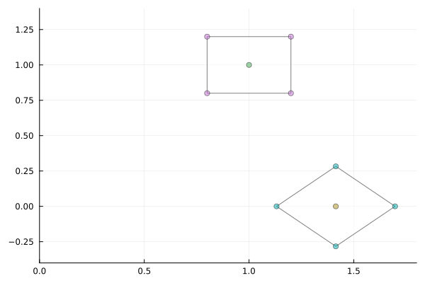
X = sample(X0, 25) .|> Singleton |> UnionSetArray

plot!(X)
plot!(linear_map(M(pi/4), X), c=:blue)     # rotate 45 degrees
plot!(linear_map(M(pi/2), X), c=:green)    # rotate 90 degrees
plot!(linear_map(M(4pi/3), X), c=:orange)  # rotate 180 degrees

plot!(X0, c=:white)
plot!(M(pi/4) * X0, c=:white)
plot!(M(pi/2) * X0, c=:white)
plot!(M(4pi/3) * X0, c=:white)
Does propagating point clouds solve the problem? Practically speaking, while we can compute the successors of any $x_0 ∈ X_0$ we still lack a global description of the set according the the given discrete recurrence.. which brings us back to the original question: how to represent the solution of the recurrence for all points in simultaneous?
Propagating zonotopes
The set representation that is most effective to this problem are zonotopes since they are closed under linear maps. Moreover, since the initial states is a hyperrectangle (thus a zonotope), we can propagate the whole set exactly (and efficiently).
We now implement the solution by propagating zonotopes.
# map X0 according to the rotation matrix
X0z = convert(Zonotope, X0)

arr = [linear_map(M(θi), X0z) for θi in range(0, 2pi, length=50)]

fig = plot(arr, ratio=1., alpha=1.)
plot!(X0, lw=2.0, ls=:dash, alpha=1., c=:white)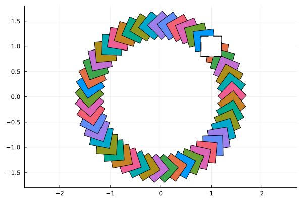
typeof(arr)Vector{Zonotope{Float64, Vector{Float64}, Matrix{Float64}}} (alias for Array{Zonotope{Float64, Array{Float64, 1}, Array{Float64, 2}}, 1})X0BallInf{Float64, Vector{Float64}}([1.0, 1.0], 0.2)convert(Zonotope, X0)Zonotope{Float64, Vector{Float64}, Matrix{Float64}}([1.0, 1.0], [0.2 0.0; 0.0 0.2])genmat(arr[1])2×2 Matrix{Float64}:
0.2 0.0
0.0 0.2(do ?Zonotope for the docstring)
genmat(arr[2])2×2 Matrix{Float64}:
0.198358 0.0255754
-0.0255754 0.198358M(2pi/50) * genmat(arr[1])2×2 Matrix{Float64}:
0.198423 0.0250666
-0.0250666 0.198423The set effectively rotates clockwise around the origin:
fig = plot(Singleton(zeros(2)))
plot!(arr[1:10], ratio=1., alpha=1.)
plot!(X0, lw=2.0, ls=:dash, alpha=1., c=:white)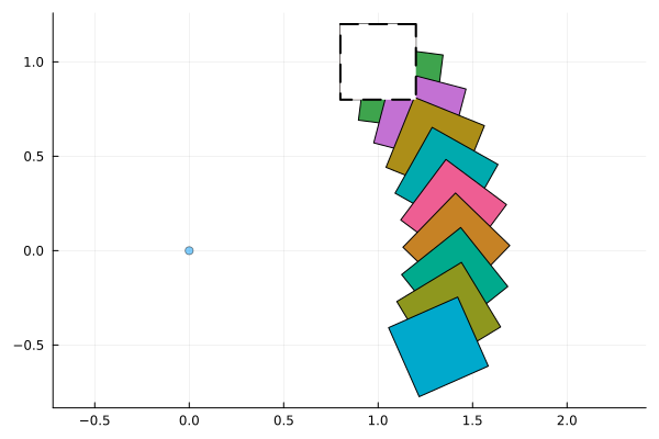
The Julia package Plots.jl has a @gif functionality that can be used to created animated gifs. The following code animates the solution at 15 frames per second (fps).
# map X0 according to the rotation matrix
X0z = convert(Zonotope, X0)

fig = plot()
anim = @animate for θi in range(0, 2pi, length=50)
    plot!(fig, linear_map(M(θi), X0z), lw=2.0, alpha=1., lab="")
    xlims!(-3, 3)
    ylims!(-2, 2)
end
gif(anim, fps=15)
Now we will use reach-sets and associate the angle $θ$ with the time field.
# propagate sets passing the time point (angle)
Rsets = [ReachSet(M(θi) * X0, θi) for θi in range(0, 2pi, length=50)]
We can pass an array of reach-sets to the plotting function:
fig = plot(Rsets, vars=(1, 2), xlab="x", ylab="y", ratio=1., c=:blue)
plot!(X0, c=:white, alpha=.6)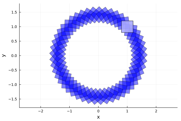
Since reach-sets have time information, we can also plot the sequence in time.
fig = plot(Rsets, vars=(0, 1), xlab="t", lab="x(t)", lw=2.0, lc=:blue, alpha=1.)
plot!(Rsets, vars=(0, 2), lab="y(t)", lw=2.0, lc=:orange, alpha=1.)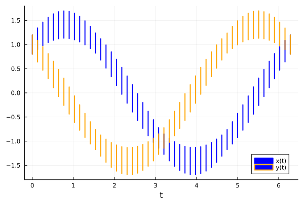
What is a flowpipe?
A flowpipe is a collection of reach-sets which behaves like their (set) union. Flowpipes attain the right level of abstraction in order to represent solutions of set-based problems.
We can instantiate a flowpipe by passing an array of reach-sets.
arr = [ReachSet(M(θi) * X0, θi) for θi in range(0, 2pi, length=50)]

F = Flowpipe(arr)
typeof(F)
Flowpipe{Float64, ReachSet{Float64, LinearMap{Float64, BallInf{Float64, Vector{Float64}}, Float64, Matrix{Float64}}}, Vector{ReachSet{Float64, LinearMap{Float64, BallInf{Float64, Vector{Float64}}, Float64, Matrix{Float64}}}}}We can plot flowpipes, and all the reach-sets are plotted with the same color.
fig = plot(F, vars=(1, 2), ratio=1.)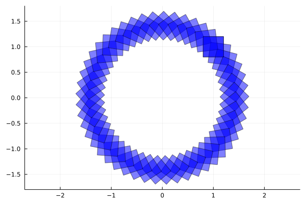
Flowpipes implement Julia's array interface.
length(F)50For instance, do F[1:3:end] to plot one every three elements:
plot!(F[1:3:end], vars=(1, 2), c=:red)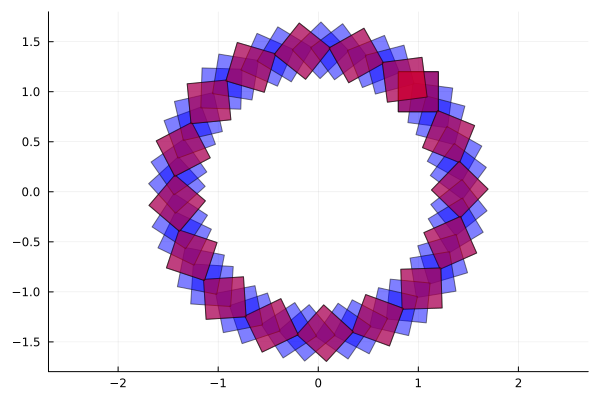
Of course, it is also possible to use the wrapped array (do array(F)) directly. However, flowpipes can be used to filter reach-sets in time, among other operations.
tspan.(F[1:5]) # time span of the first five reach-sets5-element Vector{ReachabilityAnalysis.TimeInterval{IntervalArithmetic.Interval{Float64}}}:
ReachabilityAnalysis.TimeInterval{IntervalArithmetic.Interval{Float64}}([0.0, 0.0])
ReachabilityAnalysis.TimeInterval{IntervalArithmetic.Interval{Float64}}([0.128228, 0.128229])
ReachabilityAnalysis.TimeInterval{IntervalArithmetic.Interval{Float64}}([0.256456, 0.256457])
ReachabilityAnalysis.TimeInterval{IntervalArithmetic.Interval{Float64}}([0.384684, 0.384685])
ReachabilityAnalysis.TimeInterval{IntervalArithmetic.Interval{Float64}}([0.512913, 0.512914])F(2pi) # find the reach-set at time t = 2piReachSet{Float64, LinearMap{Float64, BallInf{Float64, Vector{Float64}}, Float64, Matrix{Float64}}}(LinearMap{Float64, BallInf{Float64, Vector{Float64}}, Float64, Matrix{Float64}}([1.0 -2.4492935982947064e-16; 2.4492935982947064e-16 1.0], BallInf{Float64, Vector{Float64}}([1.0, 1.0], 0.2)), ReachabilityAnalysis.TimeInterval{IntervalArithmetic.Interval{Float64}}([6.28318, 6.28319]))We can also pick, or filter, those reach-sets whose intersection is non-empty with a given time interval.
F(2.5 .. 3.0) # returns a view4-element view(::Vector{ReachSet{Float64, LinearMap{Float64, BallInf{Float64, Vector{Float64}}, Float64, Matrix{Float64}}}}, [21, 22, 23, 24]) with eltype ReachSet{Float64, LinearMap{Float64, BallInf{Float64, Vector{Float64}}, Float64, Matrix{Float64}}}:
ReachSet{Float64, LinearMap{Float64, BallInf{Float64, Vector{Float64}}, Float64, Matrix{Float64}}}(LinearMap{Float64, BallInf{Float64, Vector{Float64}}, Float64, Matrix{Float64}}([-0.8380881048918406 0.5455349012105487; -0.5455349012105487 -0.8380881048918406], BallInf{Float64, Vector{Float64}}([1.0, 1.0], 0.2)), ReachabilityAnalysis.TimeInterval{IntervalArithmetic.Interval{Float64}}([2.56456, 2.56457]))
ReachSet{Float64, LinearMap{Float64, BallInf{Float64, Vector{Float64}}, Float64, Matrix{Float64}}}(LinearMap{Float64, BallInf{Float64, Vector{Float64}}, Float64, Matrix{Float64}}([-0.900968867902419 0.43388373911755823; -0.43388373911755823 -0.900968867902419], BallInf{Float64, Vector{Float64}}([1.0, 1.0], 0.2)), ReachabilityAnalysis.TimeInterval{IntervalArithmetic.Interval{Float64}}([2.69279, 2.6928]))
ReachSet{Float64, LinearMap{Float64, BallInf{Float64, Vector{Float64}}, Float64, Matrix{Float64}}}(LinearMap{Float64, BallInf{Float64, Vector{Float64}}, Float64, Matrix{Float64}}([-0.9490557470106686 0.3151082180236209; -0.3151082180236209 -0.9490557470106686], BallInf{Float64, Vector{Float64}}([1.0, 1.0], 0.2)), ReachabilityAnalysis.TimeInterval{IntervalArithmetic.Interval{Float64}}([2.82102, 2.82103]))
ReachSet{Float64, LinearMap{Float64, BallInf{Float64, Vector{Float64}}, Float64, Matrix{Float64}}}(LinearMap{Float64, BallInf{Float64, Vector{Float64}}, Float64, Matrix{Float64}}([-0.9815591569910653 0.19115862870137254; -0.19115862870137254 -0.9815591569910653], BallInf{Float64, Vector{Float64}}([1.0, 1.0], 0.2)), ReachabilityAnalysis.TimeInterval{IntervalArithmetic.Interval{Float64}}([2.94925, 2.94926]))We can also filter by a condition on the time span using tstart and tend:
# get all reach-sets from time t = 4 onwards
aux = F(4 .. tend(F));

length(aux)18fig = plot(F, vars=(0, 1), xlab="t", ylab="x", lw=2.0, alpha=1.)
# get all those reach-set whose time span is greater than 40
plot!(aux, vars=(0, 1), lw=2.0, lc=:red, alpha=1.)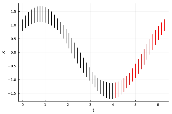
Finally, observe that set operations with flowpipes are also supported. The following example intersects the flowpipe $F$ with a half-space.
H  = HalfSpace([1, 1.], 1.) # x + y ≤ 1

Q = F ∩ H  # perform a lazy intersection

# plot the result
fig = plot(H, alpha=.3, lab="H", c=:grey)
plot!(F ∩ H, vars=(1, 2), ratio=1., lab="F ∩ H")
xlims!(-2.0, 2.0); ylims!(-2, 2.)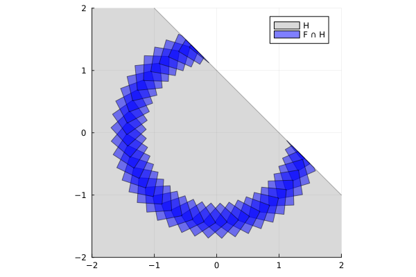
Using the solve interface for discrete problems
By default, the solve interface propagates sets in dense time (as explained in the next section). However, it is possible to propagate sets in discrete time by specifying that the approximation model should not add any bloating to the initial states, approx_model=NoBloating() to the solver used.
Exercise. Solve the linear set based recurrence in the current section using the solve interface. Hint: use the algorithm alg=GLGM06(δ=0.05, approx_model=NoBloating()) and the state matrix as specified in the following section.