Lorenz equations

Model description

This model is a system of three ordinary differential equations known as the Lorenz equations:

\[\begin{aligned} \dot{x} &= σ (y - x), \\ \dot{y} &= x (ρ - z) - y, \\ \dot{z} &= x y - β z \end{aligned}\]

The equations relate the properties of a two-dimensional fluid layer uniformly warmed from below and cooled from above. In particular, the equations describe the rate of change of three quantities with respect to time: $x$ is proportional to the rate of convection, $y$ to the horizontal temperature variation, and $z$ to the vertical temperature variation. The parameters $σ$, $ρ$, and $β$ are proportional to the Prandtl number, Rayleigh number, and certain physical dimensions of the layer itself.

using ReachabilityAnalysis

@taylorize function lorenz!(du, u, p, t)
    local σ = 10.0
    local β = 8.0 / 3.0
    local ρ = 28.0

    x, y, z = u
    du[1] = σ * (y - x)
    du[2] = x * (ρ - z) - y
    du[3] = x * y - β * z
    return du
end

Specification

The initial condition is $X_0 ∈ [0.9, 1.1] × [0, 0] × [0, 0]$, for a time span of 10.

X0 = Hyperrectangle(; low=[0.9, 0.0, 0.0], high=[1.1, 0.0, 0.0])
prob = @ivp(x' = lorenz!(x), dim:3, x(0) ∈ X0);

Analysis

We compute the flowpipe using the TMJets algorithm with $n_T=10$ and $n_Q=2$.

alg = TMJets(; abstol=1e-15, orderT=10, orderQ=2, maxsteps=50_000)
sol = solve(prob; T=10.0, alg=alg)
solz = overapproximate(sol, Zonotope);

Results

using Plots

fig = plot(solz; vars=(0, 1), xlab="t", ylab="x")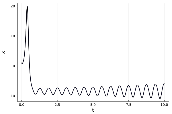

It is apparent by inspection that variable $x(t)$ does not exceed $20$ in the computed time span:

fig = plot(solz(0.0 .. 1.5); vars=(0, 1), xlab="t", ylab="x", lw=0)
plot!(fig, x -> 20.0; c=:red, xlims=(0.0, 1.5), lab="")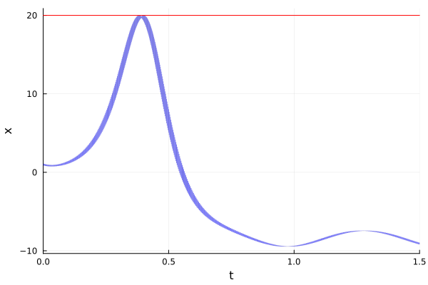

We can prove that this is the case by evaluating the support function of the flowpipe along direction $[1, 0, 0]$:

@assert ρ([1.0, 0, 0], solz(0 .. 1.5)) < 20 "the property should be proven"

ρ([1.0, 0, 0], solz(0 .. 1.5))

19.991791450503634

In a similar fashion, we can compute extremal values of variable $y(t)$:

fig = plot(solz; vars=(0, 2), xlab="t", ylab="y")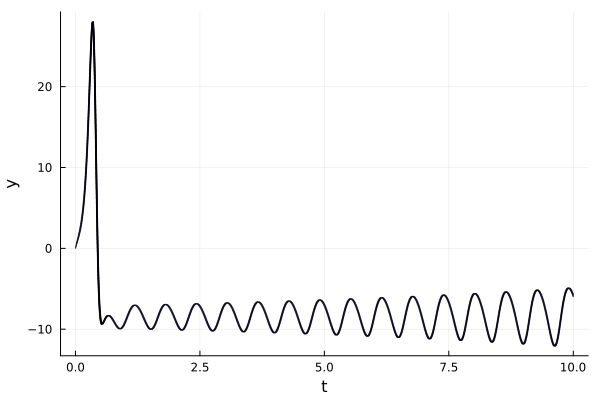

Since we have computed overapproximations of the exact flowipe, the following quantities are a lower bound on the exact minimum (resp. an upper bound on the exact maximum):

-ρ([0.0, -1.0, 0.0], solz), ρ([0.0, 1.0, 0.0], solz)

(-12.085191462246518, 28.05101124282887)

fig = plot(solz; vars=(0, 3), xlab="t", ylab="z")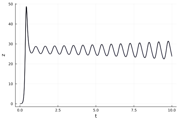

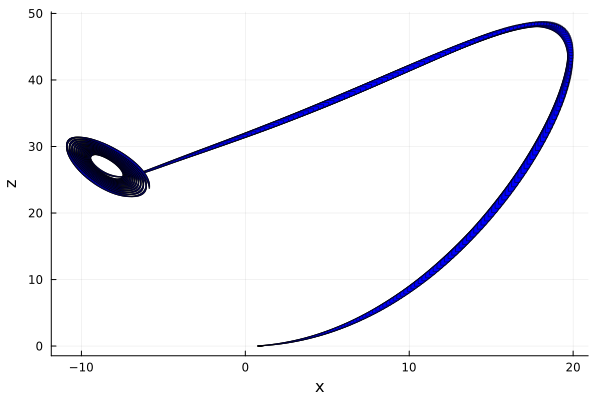
Below we plot the flowpipe projected on the $x$/$z$-plane.

fig = plot(solz; vars=(1, 3), xlab="x", ylab="z")