Spacecraft Docking

The Spacecraft Docking benchmark is a model of a docking spacecraft in 2D.

using ClosedLoopReachability
import OrdinaryDiffEq, Plots, DisplayAs
using ReachabilityBase.CurrentPath: @current_path
using ReachabilityBase.Timing: print_timed
using ClosedLoopReachability: ProjectionPostprocessing
using Plots: plot, plot!

Model

There are 4 state variables $(s_x, s_y, \dot{s}_x, \dot{s}_y)$, where $(s_x, s_y)$ is the position and $(\dot{s}_x, \dot{s}_y)$ is the velocity of the spacecraft ^[RCMGDH].

vars_idx = Dict(:states => 1:4, :controls => 5:6)

const m = 12.0
const n = 0.001027
const three_n² = 3 * n^2
const two_n = 2 * n

@taylorize function SpacecraftDocking!(dx, x, p, t)
    s_x, s_y, s_x′, s_y′, F_x, F_y = x

    dx[1] = s_x′
    dx[2] = s_y′
    dx[3] = three_n² * s_x + two_n * s_y′ + F_x / m
    dx[4] = -two_n * s_x′ + F_y / m
    dx[5] = zero(F_x)
    dx[6] = zero(F_y)
    return dx
end;

We are given a neural-network controller with 4 hidden layers of 4, 256, 256, and 4 neurons, respectively, tanh activations in the third hidden layer, and identity activations everywhere else. In particular, the first and last layer represent a pre- and postprocessing via linear maps. The controller has 4 inputs (the state variables) and 4 outputs, of which only the first two are meaningful ($F_x, F_y$).

path = @current_path("SpacecraftDocking", "SpacecraftDocking_controller.polar")
controller = read_POLAR(path)

postprocessing = ProjectionPostprocessing(1:2);

The control period is 1 time unit.

period = 1.0;

Specification

We consider a smaller uncertain initial condition than originally proposed:

X₀ = Hyperrectangle([88, 88, 0.0, 0], [1, 1, 0.01, 0.01])
U₀ = ZeroSet(2);

The control problem is:

ivp = @ivp(x' = SpacecraftDocking!(x), dim: 6, x(0) ∈ X₀ × U₀)
prob = ControlledPlant(ivp, controller, vars_idx, period;
                       postprocessing=postprocessing);

The safety specification is given as follows:

\[‖\dot{s}_x^2 + \dot{s}_y^2‖ ≤ 0.2 + 2 n ‖s_x^2 + s_y^2‖\]

A sufficient condition for guaranteed verification is to overapproximate the result via interval arithmetic.

function predicate_point(v::Union{AbstractVector,IntervalBox})
    x, y, x′, y′, F_x, F_y = v
    return sqrt(x′^2 + y′^2) <= 0.2 + two_n * sqrt(x^2 + y^2)
end

function predicate_set(R)
    return predicate_point(convert(IntervalBox, box_approximation(R)))
end

predicate(sol) = all(predicate_set(R) for F in sol for R in F)

T = 40.0
T_warmup = 2 * period;  # shorter time horizon for warm-up run

Analysis

To enclose the continuous dynamics, we use a Taylor-model-based algorithm:

algorithm_plant = TMJets(abstol=5e-1, orderT=3, orderQ=1);

To propagate sets through the neural network, we use the DeepZ algorithm:

algorithm_controller = DeepZ();

The verification benchmark is given below:

function benchmark(; T=T, silent::Bool=false)
    # Solve the controlled system:
    silent || println("Flowpipe construction:")
    res = @timed solve(prob; T=T, algorithm_controller=algorithm_controller,
                       algorithm_plant=algorithm_plant)
    sol = res.value
    silent || print_timed(res)

    # Check the property:
    silent || println("Property checking:")
    res = @timed predicate(sol)
    silent || print_timed(res)
    if res.value
        silent || println("  The property is satisfied.")
        result = "verified"
    else
        silent || println("  The property may be violated.")
        result = "not verified"
    end

    return sol, result
end;

Run the verification benchmark and compute some simulations:

benchmark(T=T_warmup, silent=true)  # warm-up
res = @timed benchmark(T=T)  # benchmark
sol, result = res.value
@assert (result == "verified") "verification failed"
println("Total analysis time:")
print_timed(res)

println("Simulation:")
res = @timed simulate(prob; T=T, trajectories=1, include_vertices=true)
sim = res.value
print_timed(res);

Flowpipe construction:
  1.117352 seconds (1.10 M allocations: 196.864 MiB, 83.30% gc time)
Property checking:
  0.004672 seconds (56.85 k allocations: 4.293 MiB)
  The property is satisfied.
Total analysis time:
  1.125494 seconds (1.16 M allocations: 202.021 MiB, 82.70% gc time)
Simulation:
  0.513139 seconds (573.64 k allocations: 50.691 MiB, 4.67% gc time)

Results

Script to plot the results:

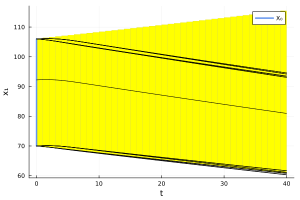
function plot_helper(vars)
    fig = plot()
    plot!(fig, sol; vars=vars, color=:yellow, lw=0, alpha=1, lab="")
    plot!(fig, project(X₀, vars); c=:cornflowerblue, alpha=0.7, lab="X₀")
    plot_simulation!(fig, sim; vars=vars, color=:black, lab="")
    return fig
end;

Plot the results:

vars = (1, 2)
fig = plot_helper(vars)
plot!(fig; xlab="x", ylab="y")
# Plots.savefig(fig, "SpacecraftDocking-x-y.png")  # command to save the plot to a file
fig = DisplayAs.Text(DisplayAs.PNG(fig))

vars = (3, 4)
fig = plot_helper(vars)
plot!(fig; xlab="x'", ylab="y'")
# Plots.savefig(fig, "SpacecraftDocking-x'-y'.png")  # command to save the plot to a file
fig = DisplayAs.Text(DisplayAs.PNG(fig))

References