Quadrotor

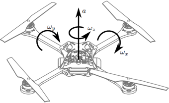
The Quadrotor benchmark is a model of a flying drone with four rotors.

using ClosedLoopReachability
import OrdinaryDiffEq, Plots, DisplayAs
using ReachabilityBase.CurrentPath: @current_path
using ReachabilityBase.Timing: print_timed
using ClosedLoopReachability: SingleEntryVector
using Plots: plot, plot!

Model

There are 12 state variables $(x_1, …, x_{12})$, where $(x_1, x_2)$ is the inertial position (north and east), $x_3$ is the altitude, $(x_4, x_5, x_6)$ is the velocity (longitudinal, lateral, vertical), $(x_7, x_8, x_9)$ is the (roll, pitch, yaw) angle, and $(x_{10}, x_{11}, x_{12})$ is the (roll, pitch, yaw) rate. The control inputs $(u_1, u_2, u_3)$ represent the torque. For more details we refer to ^[B].

vars_idx = Dict(:states => 1:12, :controls => 13:15)

const g = 9.81
const m = 1.4
const Jx = 0.054
const Jy = 0.054
const Jz = 0.104
const Cyzx = (Jy - Jz) / Jx
const Czxy = (Jz - Jx) / Jy
const Cxyz = (Jx - Jy) / Jz
const τψ = 0.0
const Tz = τψ / Jz;

The differential equations can be simplified using knowledge about the model constants:

@taylorize function Quadrotor!(dx, x, p, t)
    x₁, x₂, x₃, x₄, x₅, x₆, x₇, x₈, x₉, x₁₀, x₁₁, x₁₂, u₁, u₂, u₃ = x

    F₁ = g + u₁ / m
    Tx = u₂ / Jx
    Ty = u₃ / Jy
    sx7 = sin(x₇)
    cx7 = cos(x₇)
    sx8 = sin(x₈)
    cx8 = cos(x₈)
    sx9 = sin(x₉)
    cx9 = cos(x₉)
    sx7sx9 = sx7 * sx9
    sx7cx9 = sx7 * cx9
    cx7sx9 = cx7 * sx9
    cx7cx9 = cx7 * cx9
    sx7cx8 = sx7 * cx8
    cx7cx8 = cx7 * cx8
    sx7_cx8 = sx7 / cx8
    x4cx8 = cx8 * x₄
    xdot9 = sx7_cx8 * x₁₁

    dx[1] = (cx9 * x4cx8 + (sx7cx9 * sx8 - cx7sx9) * x₅) + (cx7cx9 * sx8 + sx7sx9) * x₆
    dx[2] = (sx9 * x4cx8 + (sx7sx9 * sx8 + cx7cx9) * x₅) + (cx7sx9 * sx8 - sx7cx9) * x₆
    dx[3] = (sx8 * x₄ - sx7cx8 * x₅) - cx7cx8 * x₆
    dx[4] = -x₁₁ * x₆ - g * sx8
    dx[5] = x₁₀ * x₆ + g * sx7cx8
    dx[6] = (x₁₁ * x₄ - x₁₀ * x₅) + (g * cx7cx8 - F₁)
    dx[7] = x₁₀ + sx8 * xdot9
    dx[8] = cx7 * x₁₁
    dx[9] = xdot9
    dx[10] = Tx
    dx[11] = Ty
    dx[12] = zero(x[12])
    dx[13] = zero(u₁)
    dx[14] = zero(u₂)
    dx[15] = zero(u₃)
    return dx
end;

We are given a neural-network controller with 3 hidden layers of 64 neurons each and sigmoid activations. The controller has 12 inputs (the state variables) and 3 outputs ($u_1, u_2, u_3$).

path = @current_path("Quadrotor", "Quadrotor_controller.polar")
controller = read_POLAR(path);

The control period is 0.1 time units.

period = 0.1;

Specification

We consider a smaller uncertain initial condition than originally proposed; specifically, the set is a hyperrectangle with 1% of the original radius:

r = [0.4, 0.4, 0.4, 0.4, 0.4, 0.4, 0, 0, 0, 0, 0, 0]  # original radius
X₀ = Hyperrectangle(zeros(12), 0.01 * r)
U₀ = ZeroSet(3);

The control problem is:

ivp = @ivp(x' = Quadrotor!(x), dim: 15, x(0) ∈ X₀ × U₀)
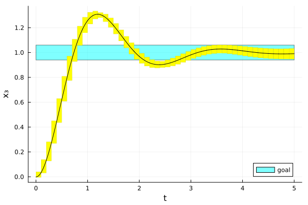
prob = ControlledPlant(ivp, controller, vars_idx, period);

The specification is to stabilize the attitude $x_3$ to the goal region $[0.94, 1.06]$ until a time horizon of 50 time units. A sufficient condition for guaranteed verification is to overapproximate the result at the end with a hyperrectangle.

goal_states = HPolyhedron([HalfSpace(SingleEntryVector(3, 15, -1.0), -0.94),
                           HalfSpace(SingleEntryVector(3, 15, 1.0), 1.06)])

predicate_set(R) = overapproximate(R, Hyperrectangle) ⊆ goal_states

predicate(sol) = predicate_set(sol[end][end])

T = 5.0
T_warmup = 2 * period;  # shorter time horizon for warm-up run

Analysis

To enclose the continuous dynamics, we use a Taylor-model-based algorithm:

algorithm_plant = TMJets(abstol=1e-1, orderT=3, orderQ=1);

To propagate sets through the neural network, we use the DeepZ algorithm:

algorithm_controller = DeepZ();

The verification benchmark is given below:

function benchmark(; T=T, silent::Bool=false)
    # Solve the controlled system:
    silent || println("Flowpipe construction:")
    res = @timed solve(prob; T=T, algorithm_controller=algorithm_controller,
                       algorithm_plant=algorithm_plant)
    sol = res.value
    silent || print_timed(res)

    # Check the property:
    silent || println("Property checking:")
    res = @timed predicate(sol)
    silent || print_timed(res)
    if res.value
        silent || println("  The property is satisfied.")
        result = "verified"
    else
        silent || println("  The property may be violated.")
        result = "not verified"
    end

    return sol, result
end;

Run the verification benchmark and compute some simulations:

benchmark(T=T_warmup, silent=true)  # warm-up
res = @timed benchmark(T=T)  # benchmark
sol, result = res.value
@assert (result == "verified") "verification failed"
println("Total analysis time:")
print_timed(res)

println("Simulation:")
res = @timed simulate(prob; T=T, trajectories=1, include_vertices=false)
sim = res.value
print_timed(res);

Flowpipe construction:
  2.753079 seconds (17.37 M allocations: 1.601 GiB, 36.53% gc time)
Property checking:
  0.000425 seconds (3.38 k allocations: 355.930 KiB)
  The property is satisfied.
Total analysis time:
  2.756976 seconds (17.37 M allocations: 1.603 GiB, 36.47% gc time)
Simulation:
  0.581457 seconds (612.87 k allocations: 43.994 MiB, 4.58% gc time)

Results

Script to plot the results:

function plot_helper(vars)
    goal_states_projected = cartesian_product(Interval(0, T),
                                              project(goal_states, [vars[2]]))
    fig = plot()
    plot!(fig, goal_states_projected; color=:cyan, lab="goal")
    plot!(fig, sol; vars=vars, color=:yellow, lw=0, alpha=1, lab="")
    plot_simulation!(fig, sim; vars=vars, color=:black, lab="")
    return fig
end;

Plot the results:

vars = (0, 3)
fig = plot_helper(vars)
plot!(fig; xlab="t", ylab="x₃")
# Plots.savefig(fig, "Quadrotor.png")  # command to save the plot to a file
fig = DisplayAs.Text(DisplayAs.PNG(fig))

References