Inverted Pendulum

The Inverted Pendulum benchmark is a classical model of motion. We consider two scenarios, which we refer to as the verification and the falsification scenario.

using ClosedLoopReachability
import OrdinaryDiffEq, Plots, DisplayAs
using ReachabilityBase.CurrentPath: @current_path
using ReachabilityBase.Timing: print_timed
using ClosedLoopReachability: SingleEntryVector, Specification, NoSplitter
using Plots: plot, plot!, xlims!, ylims!, lens!, bbox, savefig

Model

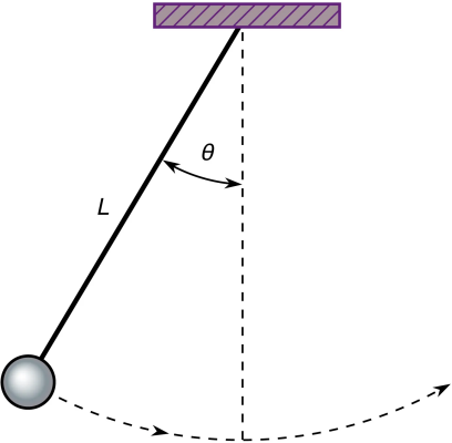
A ball of mass $m$ is attached to a massless beam of length $L$. The beam is actuated with a torque $T$. We assume viscous friction with coefficient $c$.

The governing equation of motion can be obtained as follows:

\[\ddot{θ} = \dfrac{g}{L} \sin(θ) + \dfrac{1}{m L^2} (T - c \dot{θ})\]

where $θ$ is the angle that the link makes with the upward vertical axis, $\dot{θ}$ is the angular velocity, and $g$ is the gravitational acceleration. The state vector is $(θ, \dot{θ})$. The model constants are chosen as $m = L = 0.5$, $c = 0$, and $g = 1$.

vars_idx = Dict(:states => 1:2, :controls => 3)

const m = 0.5
const L = 0.5
const c = 0.0
const g = 1.0
const gL = g / L
const mL = 1 / (m * L^2)

@taylorize function InvertedPendulum!(dx, x, p, t)
    θ, θ′, T = x

    dx[1] = θ′
    dx[2] = gL * sin(θ) + mL * (T - c * θ′)
    dx[3] = zero(T)
    return dx
end;

We are given a neural-network controller with 2 hidden layers of 25 neurons each and ReLU activations. The controller has 2 inputs (the state variables) and 1 output ($T$).

path = @current_path("InvertedPendulum", "InvertedPendulum_controller.polar")
controller = read_POLAR(path);

The control period is 0.05 time units.

period = 0.05;

Specification

The following script creates a different problem instance for the two scenarios, respectively.

function InvertedPendulum_spec(verification::Bool)
    # The uncertain initial condition is ``\dot{θ} \in [0, 0.2]``, and ``θ``
    # depends on the scenario.
    if verification
        # ``θ \in [1, 1.175]``.
        X₀ = Hyperrectangle(low=[1.0, 0], high=[1.175, 0.2])
    else
        # ``θ \in [1, 1.2]``. We choose a single point (here: the top-most one):
        X₀ = Singleton(high(BallInf([1.1, 0.1], 0.1)))
    end
    U₀ = ZeroSet(1);

    # The control problem is:

    ivp = @ivp(x' = InvertedPendulum!(x), dim: 3, x(0) ∈ X₀ × U₀)
    prob = ControlledPlant(ivp, controller, vars_idx, period);

    # The safety specification is that ``θ ∈ [0, 1]`` for ``t ∈ [0.5, 1]``
    # (i.e., the control periods ``10 ≤ k ≤ 20``). A sufficient condition for a
    # guaranteed verdict is to overapproximate the result with hyperrectangles.

    if verification
        unsafe_states = UnionSet(HalfSpace(SingleEntryVector(1, 3, -1.0), -1.0),
                                 HalfSpace(SingleEntryVector(1, 3, 1.0), 0.0))
    else
        unsafe_states = HalfSpace(SingleEntryVector(1, 3, -1.0), -1.0)
    end

    function predicate_set_safe(R)
        t = tspan(R)
        return t.hi <= 0.5 ||
            isdisjoint(overapproximate(R, Hyperrectangle), unsafe_states)
    end

    function predicate_safe(sol; silent::Bool=false)
        for F in sol
            t = tspan(F)
            if t.hi <= 0.5
                continue
            end
            for R in F
                if !predicate_set_safe(R)
                    silent || println("  Potential violation for time range $(tspan(R)).")
                    return false
                end
            end
        end
        return true
    end

    function predicate_set_unsafe(R)
        t = tspan(R)
        return t.lo >= 0.5 && t.hi <= 1.0 &&
            overapproximate(R, Hyperrectangle) ⊆ unsafe_states
    end

    function predicate_unsafe(sol; silent::Bool=false)
        for F in sol
            t = tspan(F)
            if t.hi < 0.5
                continue
            end
            for R in F
                if predicate_set_unsafe(R)
                    silent || println("  Violation for time range $(tspan(R)).")
                    return true
                end
            end
        end
        return false
    end

    if verification
        predicate = predicate_safe
    else
        predicate = predicate_unsafe
    end

    if verification
        T = 1.0
    else
        T = 11 * period  # falsification can run for a shorter time horizon
    end

    spec = Specification(T, predicate, unsafe_states)

    return prob, spec
end

T_warmup = 2 * period;  # shorter time horizon for warm-up run

Analysis

To enclose the continuous dynamics, we use a Taylor-model-based algorithm. We also use an additional splitting strategy to increase the precision. These algorithms are defined later for each scenario. To propagate sets through the neural network, we use the DeepZ algorithm:

algorithm_controller = DeepZ();

The falsification benchmark is given below:

function benchmark(prob, spec; T, algorithm_plant, splitter, verification, silent::Bool=false)
    # Solve the controlled system:
    silent || println("Flowpipe construction:")
    res = @timed solve(prob; T=T, algorithm_controller=algorithm_controller,
                       algorithm_plant=algorithm_plant, splitter=splitter)
    sol = res.value
    silent || print_timed(res)

    # Check the property:
    silent || println("Property checking:")
    if verification
        res = @timed spec.predicate(sol; silent=silent)
        silent || print_timed(res)
        if res.value
            silent || println("  The property is verified.")
            result = "verified"
        else
            silent || println("  The property may be violated.")
            result = "not verified"
        end
    else
        res = @timed spec.predicate(sol; silent=silent)
        silent || print_timed(res)
        if res.value
            silent || println("  The property is violated.")
            result = "falsified"
        else
            silent || println("  The property may be satisfied.")
            result = "not falsified"
        end
    end

    return sol, result
end

function run(; verification::Bool)
    if verification
        println("# Running analysis with verification scenario")
        algorithm_plant = TMJets(abstol=1e-9, orderT=5, orderQ=1)
        splitter = BoxSplitter([[1.1, 1.16], [0.09, 0.145, 0.18]])
    else
        println("# Running analysis with falsification scenario")
        algorithm_plant = TMJets(abstol=1e-7, orderT=4, orderQ=1)
        splitter = NoSplitter()
    end
    prob, spec = InvertedPendulum_spec(verification)

    # Run the verification/falsification benchmark:
    benchmark(prob, spec; T=T_warmup, algorithm_plant=algorithm_plant, splitter=splitter,
              verification=verification, silent=true)  # warm-up
    res = @timed benchmark(prob, spec; T=spec.T, algorithm_plant=algorithm_plant,  # benchmark
                           splitter=splitter, verification=verification)
    sol, result = res.value
    if verification
        @assert (result == "verified") "verification failed"
    else
        @assert (result == "falsified") "falsification failed"
    end
    println("Total analysis time:")
    print_timed(res)

    # Compute some simulations:
    println("Simulation:")
    trajectories = verification ? 10 : 1
    res = @timed simulate(prob; T=spec.T, trajectories=trajectories,
                          include_vertices=verification)
    sim = res.value
    print_timed(res)

    return sol, sim, prob, spec
end;

Run the analysis script for the verification scenario:

sol_v, sim_v, prob_v, spec_v = run(verification=true);

# Running analysis with verification scenario
Flowpipe construction:
  7.434132 seconds (154.16 M allocations: 6.594 GiB, 15.31% gc time)
Property checking:
  0.427641 seconds (2.15 M allocations: 99.109 MiB, 7.45% gc time, 0.00% compilation time)
  The property is verified.
Total analysis time:
  7.869467 seconds (156.31 M allocations: 6.692 GiB, 14.87% gc time, 0.00% compilation time)
Simulation:
  1.164587 seconds (6.89 M allocations: 350.970 MiB, 3.98% gc time, 0.00% compilation time)

Run the analysis script for the falsification scenario:

sol_f, sim_f, prob_f, spec_f = run(verification=false);

# Running analysis with falsification scenario
Flowpipe construction:
  0.278824 seconds (5.62 M allocations: 249.151 MiB, 18.67% gc time)
Property checking:
  Violation for time range [0.5, 0.509134].
  0.035991 seconds (32.35 k allocations: 1.754 MiB, 0.00% compilation time)
  The property is violated.
Total analysis time:
  0.322873 seconds (5.66 M allocations: 251.578 MiB, 16.13% gc time, 0.00% compilation time)
Simulation:
  0.095279 seconds (81.14 k allocations: 4.197 MiB, 0.00% compilation time)

Results

Script to plot the results:

function plot_helper(sol, sim, prob, spec, verification)
    vars = (0, 1)
    fig = plot(leg=:topright)
    lab = "unsafe"
    unsafe_states = spec.ext isa UnionSet ? spec.ext : [spec.ext]
    for B in unsafe_states
        unsafe_states_projected = cartesian_product(Interval(0.5, 1.0), project(B, [vars[2]]))
        plot!(fig, unsafe_states_projected; color=:red, alpha=:0.2, lab=lab)
        lab = ""
    end
    plot!(fig, sol; vars=vars, color=:yellow, lw=0, alpha=1, lab="")
    initial_states_projected =
        cartesian_product(Singleton([0.0]), project(initial_state(prob), [vars[2]]))
    plot!(fig, initial_states_projected; c=:cornflowerblue, alpha=1, m=:none, lw=7, lab="X₀")
    lab_sim = verification ? "" : "simulation"
    plot_simulation!(fig, sim; vars=vars, color=:black, lab=lab_sim)
    xlims!(0, spec.T)
    plot!(fig; xlab="t", ylab="θ")
    return fig
end;

Plot the results:

fig = plot_helper(sol_v, sim_v, prob_v, spec_v, true)
ylims!(fig, 0.5, 1.2)
lens!(fig, [0.49, 0.52], [0.99, 1.01]; inset=(1, bbox(0.1, 0.6, 0.3, 0.3)),
      lc=:black, xticks=[0.5], yticks=[1.0], subplot=3)
# Plots.savefig(fig, "InvertedPendulum_verification.png")  # command to save the plot to a file
fig = DisplayAs.Text(DisplayAs.PNG(fig))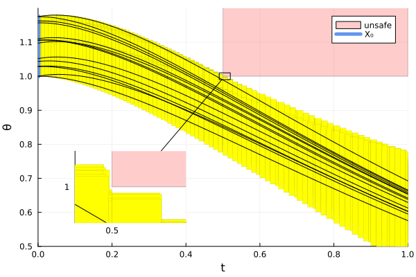

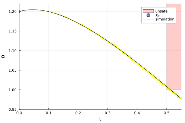
fig = plot_helper(sol_f, sim_f, prob_f, spec_f, false)
ylims!(fig, 0.95, 1.22)
# Plots.savefig(fig, "InvertedPendulum_falsification.png")  # command to save the plot to a file
fig = DisplayAs.Text(DisplayAs.PNG(fig))