Attitude Control

The Attitude Control benchmark models a rigid-body system ^[PPR].

using ClosedLoopReachability
import OrdinaryDiffEq, Plots, DisplayAs
using ReachabilityBase.CurrentPath: @current_path
using ReachabilityBase.Timing: print_timed
using Plots: plot, plot!

Model

There are 6 state variables: $(ω_1, ω_2, ω_3, ψ_1, ψ_2, ψ_3)$. The system dynamics are given as follows:

\[\begin{aligned} \dot{ω}_1 &= 0.25 (u_0 + ω_2 ω_3) \\ \dot{ω}_2 &= 0.5 (u_1 - 3 ω_1 ω_3) \\ \dot{ω}_3 &= u_2 + 2 ω_1 ω_2) \\ \dot{ψ}_1 &= 0.5 (ω₂ (ξ - ψ₃) + ω₃ (ξ + ψ₂) + ω₁ (ξ + 1)) \\ \dot{ψ}_2 &= 0.5 (ω₁ (ξ + ψ₃) + ω₃ (ξ - ψ₁) + ω₂ (ξ + 1)) \\ \dot{ψ}_3 &= 0.5 (ω₁ (ξ - ψ₂) + ω₂ (ξ + ψ₁) + ω₃ (ξ + 1)) \end{aligned}\]

where $ω = (ω_1, ω_2, ω_3)$ is the angular velocity in a body-fixed frame, $ψ = (ψ_1, ψ_2, ψ_3)$ are the Rodrigues parameters, and $ξ = ψ₁^2 + ψ₂^2 + ψ₃^2$.

vars_idx = Dict(:states => 1:6, :controls => 7:9)

@taylorize function AttitudeControl!(dx, x, p, t)
    ω₁, ω₂, ω₃, ψ₁, ψ₂, ψ₃, u₀, u₁, u₂ = x

    ξ = ψ₁^2 + ψ₂^2 + ψ₃^2

    dx[1] = 0.25 * (u₀ + ω₂ * ω₃)
    dx[2] = 0.5 * (u₁ - 3 * ω₁ * ω₃)
    dx[3] = u₂ + 2 * ω₁ * ω₂
    dx[4] = 0.5 * (  ω₂ * (ξ - ψ₃)
                   + ω₃ * (ξ + ψ₂)
                   + ω₁ * (ξ + 1))
    dx[5] = 0.5 * (  ω₁ * (ξ + ψ₃)
                   + ω₃ * (ξ - ψ₁)
                   + ω₂ * (ξ + 1))
    dx[6] = 0.5 * (  ω₁ * (ξ - ψ₂)
                   + ω₂ * (ξ + ψ₁)
                   + ω₃ * (ξ + 1))
    dx[7] = zero(u₀)
    dx[8] = zero(u₁)
    dx[9] = zero(u₂)
    return dx
end;

We are given a neural-network controller with 3 hidden layers of 64 neurons each and sigmoid activations. The controller has 6 inputs (the state variables) and 3 outputs ($u_0, u_1, u_2$).

path = @current_path("AttitudeControl", "AttitudeControl_controller.polar")
controller = read_POLAR(path);

The control period is 0.1 time units.

period = 0.1;

Specification

The uncertain initial condition is:

X₀ = Hyperrectangle(low=[-0.45, -0.55, 0.65, -0.75, 0.85, -0.65],
                    high=[-0.44, -0.54, 0.66, -0.74, 0.86, -0.64])
U₀ = ZeroSet(3);

The control problem is:

ivp = @ivp(x' = AttitudeControl!(x), dim: 9, x(0) ∈ X₀ × U₀)
prob = ControlledPlant(ivp, controller, vars_idx, period);

The safety specification is that a set of unsafe states should not be reached within 3 time units. A sufficient condition for guaranteed verification is to overapproximate the result with hyperrectangles.

unsafe_states = cartesian_product(
    Hyperrectangle(low=[-0.2, -0.5, 0,   -0.7, 0.7, -0.4],
                   high=[0,   -0.4, 0.2, -0.6, 0.8, -0.2]),
    Universe(3))

predicate(sol) = isdisjoint(overapproximate(sol, Hyperrectangle), unsafe_states);

T = 3.0
T_warmup = 2 * period;  # shorter time horizon for warm-up run

Analysis

To enclose the continuous dynamics, we use a Taylor-model-based algorithm:

algorithm_plant = TMJets(abstol=1e-4, orderT=5, orderQ=1);

To propagate sets through the neural network, we use the DeepZ algorithm:

algorithm_controller = DeepZ();

The verification benchmark is given below:

function benchmark(; T=T, silent::Bool=false)
    # Solve the controlled system:
    silent || println("Flowpipe construction:")
    res = @timed solve(prob; T=T, algorithm_controller=algorithm_controller,
                       algorithm_plant=algorithm_plant)
    sol = res.value
    silent || print_timed(res)

    # Check the property:
    silent || println("Property checking:")
    res = @timed predicate(sol)
    silent || print_timed(res)
    if res.value
        silent || println("  The property is satisfied.")
        result = "verified"
    else
        silent || println("  The property may be violated.")
        result = "not verified"
    end

    return sol, result
end;

Run the verification benchmark and compute some simulations:

benchmark(T=T_warmup, silent=true)  # warm-up
res = @timed benchmark(T=T)  # benchmark
sol, result = res.value
@assert (result == "verified") "verification failed"
println("Total analysis time:")
print_timed(res)

println("Simulation:")
res = @timed simulate(prob; T=T, trajectories=10, include_vertices=false)
sim = res.value
print_timed(res);

Flowpipe construction:
  1.474104 seconds (5.66 M allocations: 483.964 MiB, 60.21% gc time)
Property checking:
  0.011338 seconds (117.67 k allocations: 9.516 MiB)
  The property is satisfied.
Total analysis time:
  1.489019 seconds (5.78 M allocations: 494.345 MiB, 59.61% gc time)
Simulation:
  0.613352 seconds (996.81 k allocations: 74.591 MiB)

Results

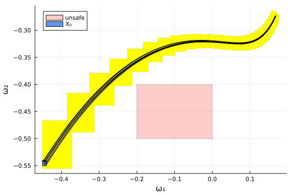
Script to plot the results:

function plot_helper(vars)
    fig = plot()
    plot!(fig, project(unsafe_states, vars); color=:red, alpha=:0.2,
          lab="unsafe", leg=:topleft)
    plot!(fig, sol; vars=vars, color=:yellow, lw=0, alpha=1, lab="")
    plot!(fig, project(X₀, vars); c=:cornflowerblue, alpha=1, lab="X₀")
    plot_simulation!(fig, sim; vars=vars, color=:black, lab="")
    return fig
end;

Plot the results:

vars = (1, 2)
fig = plot_helper(vars)
plot!(fig; xlab="ω₁", ylab="ω₂")
# Plots.savefig(fig, "AttitudeControl.png")  # command to save the plot to a file
fig = DisplayAs.Text(DisplayAs.PNG(fig))

References