Tutorial
This tutorial will teach you how to use RangeEnclosures. First, we will give a basic overview of the package and its functionalities. Next, we will discuss in more detail how to use the package in different scenarios (1D, higher dimension, using algorithms from external libraries, etc.).
Setup
Assuming you have installed Julia, you can install the package from the Julia REPL with the following lines.
using Pkg
Pkg.add("RangeEnclosures")
Then you can load the package in the standard way.
using RangeEnclosuresOverview
RangeEnclosures is used to bound the range of a given function f. The main function provided by this package is enclose, and its basic usage is the following.
enclose(f, D, solver; kwargs...)where
fis the function whose range we want to bound,Dis the domain over which we want to compute the range,solveris the solver used to compute the range (which is optional; if not specified, the package will default to theNaturalEnclosuresolver), andkwargs...are possible keyword arguments used by the solver.
The solvers can be divided into two families: direct solvers, which compute the range enclosure over the whole domain, and iterative solvers, which recursively split the domain into smaller subdomains to get a more accurate estimate. A detailed list of available solvers can be found here.
Usage Examples
A one-dimensional example
Suppose we want to compute the range of the function
\[f(x) = -\sum_{k=1}^5kx\sin\left(\frac{k(x-3)}{3}\right)\]
over the domain $D = [-10, 10]$.
If we call enclose without specifying the solver, it will evaluate $f(D)$ using plain interval arithmetic (this is called natural enclosure), as the following example shows.
f(x) = -sum(k*x*sin(k*(x-3)/3) for k in 1:5)
D = interval(-10, 10)
R = enclose(f, D)
[-150.0, 150.0]_com_NGGenerally, using natural enclosures leads to unpleasantly large overestimates, which is due to the dependency problem. To overcome this, you may want to use some other solvers in your application. The next example bounds the range using the BranchAndBoundEnclosure solver.
Rbb = enclose(f, D, BranchAndBoundEnclosure())[-56.4241, 34.9884]_trv_NGAs you can see, the result is much tighter now, while still being rigorous! The results can be visualized using Plots.jl.
using Plots
using RangeEnclosures: inf, sup

function plot_box!(fig, box::IntervalBox{2}; label, alpha)
    (x, y) = box
    x = [inf(x), sup(x), sup(x), inf(x)]
    y = [inf(y), inf(y), sup(y), sup(y)]
    plot!(fig, x, y, seriesalpha=alpha, seriestype=:shape, label=label)
    x, y
end

fig = plot(xlabel="x", ylabel="f(x)", legendfontsize=12, tickfontsize=12,
           xguidefont=font(15, "Times"), yguidefont=font(15, "Times"))
plot_box!(fig, IntervalBox(D, R), label="natural enclosure", alpha=0.5)
plot_box!(fig, IntervalBox(D, Rbb), label="branch and bound", alpha=1)
plot!(fig, f, -10, 10, lw=2, c=:black, label="f")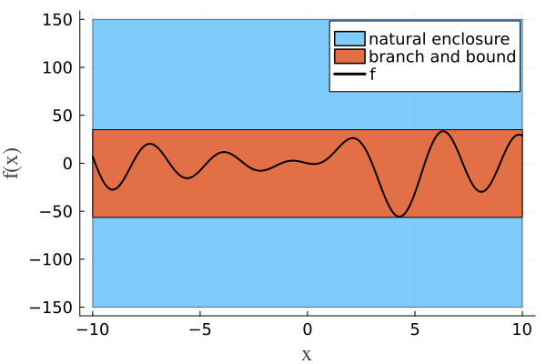
Tuning parameters
Some solvers have parameters that can be tuned. For example, looking at the BranchAndBoundEnclosure documentation, we can see that it has two parameters, tol and maxdepth. If you want to use different values from the default ones, you can pass the parameters as keyword arguments to the solver constructor. For example, you can limit the depth of the search tree to 6 the following way:
enclose(f, D, BranchAndBoundEnclosure(maxdepth=6))[-61.1288, 57.1972]_trv_NGGenerally, tuning parameters can be a good idea to achieve the desired accuracy tradeoff in your application.
Combining different solvers
Sometimes there is no strictly "best" solver, as one solver might give a tighter estimate of the range's upper bound and another solver might give a tighter estimate on the lower bound. In this case, the results can be combined by taking the intersection. For example, let us consider the function $g(x) = x^2 - 2x + 1$, which we want to bound over the domain $D_g = [0, 4]$. Let us first use plain interval arithmetic:
g(x) = x^2 - 2*x + 1
Dg = interval(0, 4)
enclose(g, Dg, NaturalEnclosure()) # this is equivalent to enclose(g, Dg)
[-7.0, 17.0]_com_NGNow let us bound the range using the MeanValueEnclosure solver, which uses the mean-value form of the function:
enclose(g, Dg, MeanValueEnclosure())[-11.0, 13.0]_com_NGAs you can see, there is no clear winner and a better enclosure could be obtained by taking the intersection of the two results. This can be easily done in one command by passing a vector of solvers to enclose:
enclose(g, Dg, [NaturalEnclosure(), MeanValueEnclosure()])[-7.0, 13.0]_trv_NGUsing solvers based on external libraries
Some of the available solvers are implemented in external libraries. To keep the start-up time of RangeEnclosures.jl low, these libraries are not imported by default. To use more solvers, these libraries need to be manually loaded. For example, suppose we want to bound the previous function using the Moore-Skelboe algorithm. Trying the following will fail:
enclose(f, D, MooreSkelboeEnclosure())ERROR: AssertionError: package 'IntervalOptimisation' not loaded (it is required for executing `enclose`)
...This is because the algorithm is implemented in IntervalOptimisation.jl and to use it you need to load that package first (note that you need to have it installed before loading it). Let us fix our example.
using IntervalOptimisation
enclose(f, D, MooreSkelboeEnclosure())
[-55.6016, 33.4161]_comBounding multivariate functions
While our previous examples were in one dimension, the techniques generalize to multivariate functions $\mathbb{R}^n\rightarrow\mathbb{R}$, the only difference is that the domain, instead of being an interval, should be an IntervalBox. For example, consider the function
\[h(x_1, x_2) = \sin(x_1) - \cos(x_2) - \sin(x_1)\cos(x_1)\]
over the domain $D_h = [-5, 5] \times [-5, 5]$. An enclosure can be computed as follows.
h(x) = sin(x[1]) - cos(x[2]) - sin(x[1]) * cos(x[1])
Dh = IntervalBox(interval(-5, 5), interval(-5, 5))
Rh = enclose(h, Dh, BranchAndBoundEnclosure())
[-2.71144, 2.71313]_trvWe can visualize the result with the following script.
x = y = -5:0.1:5
f(x, y) = h([x, y])
fig = plot(legend=:none, size=(800, 800), xlabel="x", ylabel="y", zlabel="h(x,y)",
           tickfontsize=18, guidefont=font(22, "Times"), zticks=[-2, 0, 2])
surface!(fig, x, y, [inf(Rh) for _ in x, _ in y], α=0.4)
surface!(fig, x, y, f.(x', y), zlims=(-4, 4))
surface!(fig, x, y, [sup(Rh) for _ in x, _ in y], α=0.4)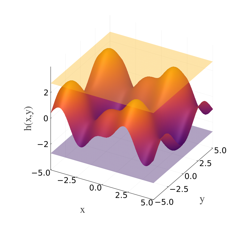
Adding a new enclosure algorithm
To add a new enclosure algorithm, or solver, just add a corresponding struct (let us call it MyEnclosure) and extend the method enclose, as the following code snippet demonstrates.
using RangeEnclosures
import RangeEnclosures: enclose
using RangeEnclosures: Interval, IntervalBox

struct MyEnclosure end

function enclose(f::Function,
                 D::Union{Interval,IntervalBox},
                 solver::MyEnclosure; kwargs...)
    # solver-specific implementation
end
Note that the domain D can be of type Interval for univariate ($n = 1$) functions or of type IntervalBox for multivariate ($n > 1$) functions.